Chapter 10 Improving Metric Sensitivity

There are two important aspects for a metric: its directionality and sensitivity (A. Deng and Shi 2016). The directionality of a metric tells us how to interpret the movement of it. In other words, the movement of the metric positively or negatively should be able to tell us something good or bad happened. Metrics without a clear directionality may still be useful for other purposes such as to provide side information for another main metric, but they are unfit to aid directly in decision making. Sensitivity of a metric reflects how likely we can move the metric in an experiment. The more sensitive the metric, the more actionable the metric is. A metric can have very good directionality but if it rarely moves in a typical A/B tests, it is barely useful.

Directionality is largely inherent from the design and definition of the metric itself. Sensitivity, on the other hand, not only depends on the metric definition, but also the experiment design and statistical method used for inference.

10.1 Metric Sensitivity Decomposition

By definition, metric sensitivity reflects how easy a metric can be moved in an A/B test. What do we mean by move a metric? We have learned in Chapter 8 that being a statistic, the movement of a metric need to be interpreted in a statistical way. For a predefined confidence level $\alpha$, we declare a metric moved if the null hypothesis of zero ATE is rejected at $\alpha$ level. That is, the p-value of a two-sided null hypothesis test is less than $\alpha$, or equivalently the two-sided $1-\alpha$ confidence interval excludes zero. Under this definition, the probability of a metric moved in an A/B test is given by:

\[\begin{equation} P(\text{Reject $H_0$}) = \int P(\text{Reject $H_0$}|\delta)dP(\delta)\,, \tag{10.1} \end{equation}\] where $\delta$ is the true ATE and the integration is to average over a distribution of treatment effect $\delta$. From Equation (10.1) it is easy to see the sensitivity can be decomposed into two factors:

The statistical power: The probability of rejecting the null hypothesis given a fixed ATE $\delta$.
The distribution of the true ATE $\delta$.

Therefore, to improve the sensitivity, we can either improve the statistical power, or change the effect $\delta$ itself. This can also be seen from the z-score \[ \frac{\Delta}{\sqrt{\sigma_t^2/n_t + \sigma_c^2/n_c}} \,, \] whose mean value is \[ \frac{\delta}{\sqrt{\sigma_t^2/n_t + \sigma_c^2/n_c}} \,. \] On average, to increase the value of the absolute value of z-score, we either increase the numerator $|\delta|$ — that is to change the distribution of $\delta$, or decrease the denominator to increase statistical power. When we found a metric hard to move in experiments and seeks way to improve its sensitivity, it is crucial to understand which one of the two factors is the main issue.

In most cases lacking sensitivity of a metric is mainly due to low statistical power, and we should focus on reducing variance of the metric. We can reduce variance of the metric by either increasing the sample size of each variants, or coming up with a more efficient ATE estimator that has less variance than the standard $\Delta$. Increasing sample size can be done by running experiment at a larger traffic percentage for each variant group, e.g., using 20% traffic for both treatment and control instead of 5%. This approach is limited to 50% treatment and 50% control as the maximum, and even less traffic per group if we run multiple treatments concurrently. Another common way of increasing sample size is to run experiments longer. Two week experiment typically have more users than one week experiment. However, as mentioned in Section 7.1, when we change experiment period from one week to two weeks, the population mixture for heavy user and casual user also changes, as well as the distribution of metrics. As the result metric variance may not decrease, as shown in Figure 7.1. Nevertheless, for most metrics running experiment longer increases statistical power. Reducing metric variance via more efficient ATE estimator is always a good thing to do whenever possible to make sure we don’t leave any “free” sensitivity on the table. This is be our topic in Section 10.2.

When low sensitivity is due to the numerator — the $\delta$, it means the distribution of $\delta$ is very close to 0 and can be treated as practically 0 most of the time. The first question we should be asking is what is the triggering rate of the change we are testing. If the change we make by design will only affect a very small proportion of the population, then majority of the users will not have any treatment effect and including them in the analysis will only dilute the $\delta$. By zooming into those users who are affected by the treatment, we can increase $|\delta|$ and improve sensitivity. Analyzing only triggered population is called triggered analyses. When doing triggered analysis, it is

10.2 Variance Reduction

So far we have been using the simple difference of sample averages $\Delta$ to estimate the ATE $\delta$. Randomization guarantees it is unbiased, that is $E(\Delta) = \delta$. The statistical power of the two sample test based on $\Delta$ relies on its variance $\mathrm{Var}(\Delta)$. Reducing its variance increases statistical power and the sensitivity of the metric.

Usually, there is a trade-off between variance and bias, so called bias-variance trade-off. However, as we will see, there is a way to reduce the variance without introducing any bias. Statisticians calls this efficiency augmentation (Tsiatis 2006). Efficiency augmentation here means more accurate estimation using the same amount of information or sample size. In other words, we seek to come up with a new estimator $\Delta^*$ to replace $\Delta$ that is still unbiased and with smaller variance. We show a simple and powerful idea based on variance reduction using control variates from Monte Carlo simulation. The general theory of regression adjustment and semiparametric efficiency augmentation is closely related to the idea of doubly robust estimation in Section 4.9.

10.2.1 Control Variates and CUPED

In the context of Monte Carlo simulation, we face a similar problem of estimate the mean $\mathrm{E}(Y)$ of a random variable $Y$ for which we can simulate (draw sample) from. The naive Monte Carlo estimator is the sample mean $\overline{Y}$, similar to the naive ATE estimator $\Delta$. Control variates provide an alternative Monte Carlo estimator with smaller variance. To do that, we need another random variable $X$ with known mean $\mu_x=\mathrm{E}(X)$. For any fixed value of $\theta$, the following is also an unbiased estimator for $\mathrm{E}(Y)$: \[ \widehat{Y}_{cv}:=\overline{Y} - \theta \overline{X} + \theta \mu_x\,. \] The unbiasedness of $\widehat{Y}_{cv}$ is due to the fact that last two terms on the right hand side cancels with each other since $\mathrm{E}(\overline{X})= \mu_x$. Also note that this estimator requires $\mu_x$ to be known to even be defined.

The variance of this newly created estimator $\widehat{Y}_{cv}$ is \[\begin{align*} \mathrm{Var} (\widehat{Y}_{cv}) &= \mathrm{Var} (\overline{Y} - \theta \overline{X}) = \mathrm{Var} (Y-\theta X)/n \\ &=\frac{1}{n} (\mathrm{Var} Y) + \theta^2\mathrm{Var} (X) - 2\theta\mathrm{Cov} (Y,X))\,. \end{align*}\] Note that $\mathrm{Var} (\widehat{Y}_{cv})$ is minimized when we choose \[\begin{align} \theta = \mathrm{Cov}(Y,X)/\mathrm{Var}(X) \tag{10.2} \end{align}\] and with this optimal choice of $\theta$, we have \[ \mathrm{Var} (\widehat{Y}_{cv}) = \mathrm{Var}(\overline{Y}) (1- \rho^2) \,, \] where $\rho = \mathrm{Cor} (Y,X)$ is the correlation between $Y$ and $X$. That is \[ \frac{\mathrm{Var} (\widehat{Y}_{cv})}{\mathrm{Var}(\overline{Y})} = 1 - \rho^2 \,. \] That is, the variance is reduced by a factor of $\rho^2$! The larger $\rho$, the better the variance reduction.

The single control variate case can be easily generalized to include multiple variables. It is interesting to point out the connection with linear regression. The optimal $\theta$ turns out to be the ordinary least square (OLS) solution of regressing (centered) $Y$ on (centered) $X$, which in multiple variable case has variance \[\begin{align*} \mathrm{Var} (\widehat{Y}_{cv}) &= \mathrm{Var}(\overline{Y}) (1- R^2) \,, \end{align*}\] with $R^2$ being the proportion of variance explained coefficient from the linear regression.

It is also possible to use nonlinear adjustment. Instead of allowing only linear adjustment, we can minimize variance in a more general functional space. Let \[\begin{align} \widehat{Y}_{cv} = \overline{Y} - \overline{f(X)} + \mathrm{E}(f(X)), \tag{10.3} \end{align}\] and then try to minimize the variance of . It can be shown that the regression function $\mathrm{E} (Y|X)$ gives the optimal $f(X)$.

Exercise: Prove $f(X) = \mathrm{E} (Y|X)$ is the optimal control variates for $Y$ using $X$.

So far we have been looking at one sample mean and assume the mean of control variate $\mu_x$ to be known. Utilizing control variates to reduce variance is a very common technique in Monte Carlo simulation (Asmussen and Glynn 2008). The difficulty of applying it usually boils down to finding a control variate $X$ that is highly correlated with $Y$ and at the same time has known $\mathrm{E}(X)$.

Alex Deng et al. (2013) made the observation that in a randomized experiment, we don’t need to know $\mu_x$ to use $X$ as control variate because we care about the ATE, not the two means $\mathrm{Y^{(t)}}$ and $\mathrm{Y^{(c)}}$ for treatment and control groups. If we replace $\overline{Y^{(t)}}$ by $\overline{Y^{(t)}_{cv}}$ and $\overline{Y^{(c)}}$ by $\overline{Y^{(c)}_{cv}}$, and then define \[\begin{align*} \Delta^* &:= \overline{Y^{(t)}_{cv}} - \overline{Y^{(c)}_{cv}} \\ &= \Delta(Y) - \theta \Delta(X) + \theta (\mathrm{E}(X^{t})-\mathrm{E}(X^{c}))\,. \end{align*}\] Here $\Delta(Y) = \overline{Y^{t}} - \overline{Y^{c}}$ and $\Delta(X) = \overline{X^{t}} - \overline{X^{c}}$ are simple difference of sample means. From Equation (10.4) it is apparent that if $\mathrm{E}(X^{t})=\mathrm{E}(X^{c}))$, the last term disappear and \[\begin{equation} \Delta^* = \Delta(Y) - \theta \Delta(X) \tag{10.4}\,. \end{equation}\]

In a few elementary steps, we have achieved wonder. This new $\Delta^*$ in Equation (10.4) does not involve any unknown mean $\mathrm{E}(X^{t})$ or $\mathrm{E}(X^{c})$. Moreover, its variance can be greatly reduced comparing to the original ATE estimator $\Delta$ thanks to control variate $X$. The only requirement is the control variates $X$ we picked need to satisfy the condition \[ \mathrm{E}(X^{t})=\mathrm{E}(X^{c}))\,. \] that is, the ATE on $X$ must be zero. These kind of $X$ are abundant in practice, because a treatment cannot possibly impact anything observed before an experiment unit get exposed to the treatment. Alex Deng et al. (2013) calls these pre-experiment variables and named the simple procedure described so far CUPED (Controlled experiment Using Pre-Experiment Data), and demonstrated the effectiveness of using the same metric data for the pre-experiment period as control variates performs well in practice. Figure 10.1 shows the variance of a metric reduced by more than 50%. With only half of the original sample size, $\Delta^*$ of CUPED produces more statistical power than estimating ATE by $\Delta$.

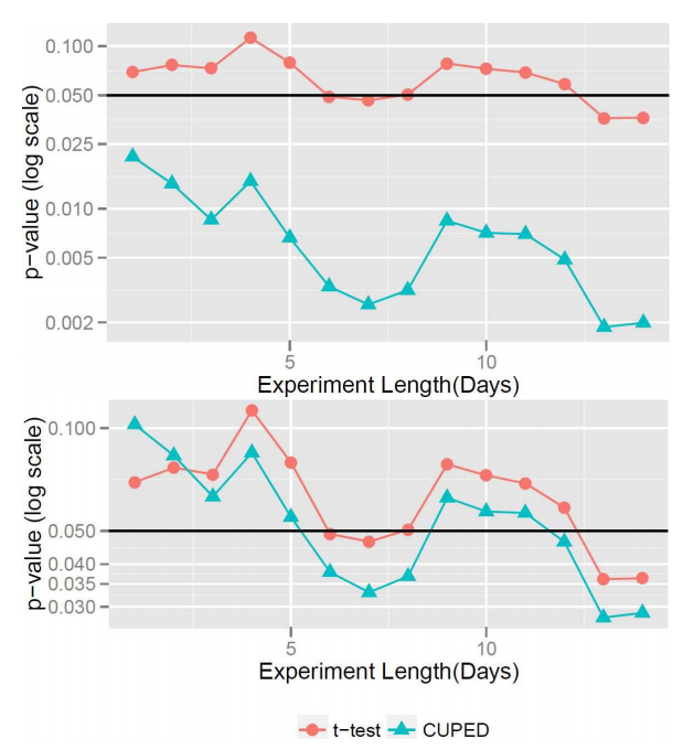
Figure 10.1: Variance Reduction in Action for a real experiment. Top: p-value. Bottom: p-value when using only half the users for CUPED.

A few important remarks:

Optimal $\theta$ is $\mathrm{Cov}(Y,X)/\mathrm{Var}(X)$ for control variates. In CUPED, we have treatment and control groups. Should we use treatment or control group to define the optimal $\theta$? The answer is it usually does not matter much. Note that the CUPED estimator $\Delta^*$ is unbiased for any fixed value of $\theta$, and different $\theta$ merely affect variance reduction rate. As long as the treatment effect is not too big, the optimal $\theta$ for the two groups are very close and it does not make a lot of difference which one to choose. If needed, one can optimize $\theta$ to minimize the variance of $\Delta^*$ directly. The minimizer of $\mathrm{Var}(\Delta^*)$ is \[ \frac{\mathrm{Cov}(\overline{Y^{t}},\overline{X^{t}})+\mathrm{Cov}(\overline{Y^{c}},\overline{X^{c}})}{\mathrm{Var}(\overline{X^{t}})+\mathrm{Var}(\overline{X^{c}})}\,. \] Another choice is to use pooled data of treatment and control to compute $\theta$. In Section 10.2.2 we will use results from more general semiparametric theory to bring a much clearer picture.
Equation (10.4) can be trivially extended to nonlinear adjustment: \[\begin{equation} \Delta^* := \overline{Y^{(t)}_{cv}} - \overline{Y^{(c)}_{cv}} = \Delta(Y) - \Delta(f(X)) \tag{10.5}\,. \end{equation}\] Similar to control variates, the closer $f(X)$ to $\mathrm{E}(Y|X)$, the better the variance reduction.
Pre-experiment data does not literally means data collected before the experiment begins. It can be anything before the triggering of the treatment intervention. For example, the day-of-week a user is first observed in the experiment is independent of the experiment itself, as well as the age, gender, browser and the device a user uses.
Control variates $X$ can be categorical (discrete) or continuous. When $X$ is categorical, we can use one-hot encoder to create dummy binary variables, and CUPED can be seen as post-stratification adjustment, which is shown to be asymptotically as efficient as doing actual blocking (stratified sampling) (Miratrix, Sekhon, and Yu 2013).
For some choice of $X$, it might be not be well-defined for a subset of experiment units. For example, new users just appeared during the experiment do not exist before the experiment period and the pre-experiment period metric value for them are simply not defined. In such cases, Alex Deng et al. (2013) proposed to impute with $0$ and at the same time also include an binary indicator variate to indicate whether a unit has valid pre-experiment and use both in a multiple regression version of CUPED.
There is a deep connection between control variates and linear regression. However, control variates method does not actually assume any linear relationship between $X$ and $Y$. The linear regression and the optimal $\theta$ being solution of OLS is simply a working model. The extension to nonlinear $f(X)$ makes it clear that the working model can be any model and the quality of the model only affects the variance reduction rate. Therefore, CUPED is not the same as directly fitting a linear regression with treatment assignment indicator and predictors $X$, despite the resemblance. In the next section we will use a more general semiparametric model to emphasize the distinction.

10.2.2 General Regression Adjustment and Doubly Robust Estimation

There is a clear resemblance between CUPED and linear regression. Let $A_i$ be the binary treatment assignment indicator of the ith experiment unit. Consider the following two common linear regression models: \[\begin{equation} Y_i = \alpha + \delta A_i + \beta X_i + \epsilon_i \tag{10.6} \,, \end{equation}\] and \[\begin{equation} Y_i = \alpha + \delta A_i + \beta X_i + (\gamma X_i)A_i + \epsilon_i \tag{10.7}\,. \end{equation}\] Under the standard linear regression model assumptions, the regressors $X$ and $A$ are considered to be fixed, the residual $\epsilon_i$ are assumed to be i.i.d. with a normal distribution. The only random component in the underlying data-generating-process are from the residuals alone. $\alpha+\beta X$ is the prediction for $Y$ in the control group based on $X$. $\delta$ is the average treatment effect and $\gamma X_i$ in the second model is the linear treatment effect adjustment that allows the conditional treatment effect $\mathrm{E}(\tau|X)$ to be a linear function of $X$. Fitting the linear model to get estimators of those coefficients and their sampling distributions are also known as Analysis of (Co)Variances (ANOVA/ANCOVA). We call the first model ANCOVA1 and the second ANCOVA2.

Both models are widely used in two group comparison for both experiment data and also observational data. Many have pointed out the efficiency gain from the regression model to increase accuracy of estimating the average treatment effect $\delta$. Nevertheless, it is obvious that the linear model is too restrictive. The data-generating-process for real world problems will involve random $X$ and $A$; the true regression $\mathrm{E}(Y|X,A)$ will unlikely be linear, so $\epsilon$ may not even satisfy $\mathrm{E}(\epsilon|X) = 0$, let alone i.i.d. normally distributed.

Freedman (Freedman 2008) criticized the practices of using parametric linear regression theory on experimentation data, stating: “randomization does not justify the models, bias is likely; nor are the usual variance calculations to be trusted.” Using Neyman’s complete randomization with potential outcomes (see Section 3.1), Freedman avoid postulating a parametric model for $(Y(T),Y(C),X)$ by treating them as fixed and the only random component is the treatment assignment $A$. Asymptotic and finite sample theories for the ANCOVA1 model was given in Freedman (2008); and a following work Lin (2013) studied the ANCOVA2 model.

Here we follow the independent randomization model (Section 3.2) and assume $(Y,X,A)$ are independently sampled from a super population. The model we use is general. The joint distribution of $(Y,X,A)$ are allowed to be anything except the restriction that $A$ is result of independent randomization. That is, the joint density has a natural decomposition as \[\begin{equation} p(y,x,a) = p_y(y|x,a)p_a(a|x)p(x) \, \tag{10.8} \end{equation}\] and $p_a(a|x)$ is known to be the Bernoulli density $p^a(1-p)^{(1-a)}$ with fixed treatment probability $p$. This kind of model with a combination of both parametric and nonparametric components are called semiparametric model.

The target of the inference is to estimate the ATE \[ \delta = \mathrm{E}(Y|A = 1) - \mathrm{E}(Y|A=0)\,. \] Unlike in a parametric model where the target of inference is either one of the model parameters or a function of them, for semiparametric model, the inference can be any functional of the distribution.

For large sample, asymptotic theories exist for semiparametric model just like parametric model. It can be shown that all reasonable consistent and asymptotically normal estimators for $\delta$ are either exactly or asymptotically equivalent to this form: \[\begin{equation} \overline{Y^{(t)}} - \overline{Y^{(c)}} + \frac{1}{n}\sum \left((A_i - p)h(X_i)\right) \tag{10.9} \end{equation}\] for a function $h$ of $X$.

A rigorous explanation is beyond our scope and can be found in Tsiatis (2006), Van der Vaart (2000) or Robins and Rotnitzky (1995). Here we just state some general results focusing on high level intuitions. Asymptotic theory for semiparametric models focus on only regular and asymptotically linear estimators (RAL). Regularity condition is to avoid pathological estimators whose behavior can vary dramatically in the neighborhood of the ground truth value, as exemplified by Hodges’ estimator (Van der Vaart 2000). Consistent RAL estimators represents all reasonable estimators of interest with nice properties such as asymptotical normality, including MLE for parametric models, M-estimator and Z-estimator.

Semiparametric theory guarantees that all consistent RAL is asymptotically equivalent to an estimator of the form \[ \overline {\psi(Y,X,A)} + \overline{h(Y,X,A)}\,, \] where $\overline{\psi(Y,X,A)}$ is any consistent RAL estimator and $h(Y,X,A)$ is from a linear subspace of the Hilbert space of mean-zero finite variance random functions. This linear subspace, denoted by $\mathcal{T}^{\perp}$, is the orthogonal component of the tangent space $\mathcal{T}$. The tangent space for a parametric model can be defined as the linear subspace spanned by score functions. For a semiparametric model, the tangent space contains the tangent space of any parametric submodel – that is, a parametric model whose distribution is also included in the semiparametric model.

For our purpose, we already have a consistent RAL. The naive $\Delta$ estimator $\overline{Y^{(t)}} - \overline{Y^{(c)}}$ is asymptotically equivalent to \[ \overline {\frac{AY}{p} - \frac{(1-A)Y}{1-p}}\,. \] Turns out that the linear space $\mathcal{T}^{\perp}$ has a very simple form. It contains all mean-zero finite variance functions of $h(A,X)$ such that \[ \mathrm{E}(f(A,X)|X) = 0\,. \] Since $f(A,X)$ is $f(1,X)$ with probability $p$ and $f(0,X)$ with probability $1-p$, the above condition together with the independence of $A$ and $X$ entails \[ f(A,X) = \frac{A-p}{1-p}f(1,X) \,. \] Let $h(X)= f(1,X)/(1-p)$, we have shown Equation (10.9) characterizes all consistent RAL for ATE $\delta$.

Exercise: Show $\overline{Y^{(t)}} - \overline{Y^{(c)}}$ is asymptotically equivalent to $\overline {\frac{AY}{p} - \frac{(1-A)Y}{1-p}}$. Show $f(A,X) = \frac{A-p}{1-p}f(1,X)$ if $\mathrm{E}(f(A,X)|X) = 0$ and $A$ is independent Bernoulli(p).

Because $\mathrm{E}\left((A_i - p)h(X_i)\right) = 0$, Equation (10.9) can be seen as a sum of any consistent RAL estimator and another estimator of $0$. This is similar to CUPED where we augment naive ATE estimator $\Delta$ by $\theta\Delta(X)$. Like in CUPED we optimize $\theta$ to minimize variance, here we can minimize the variance of (10.9) to find the optimal functional form of $h(X)$.

Using the asymptotic equivalent form $\overline {\frac{AY}{p} - \frac{(1-A)Y}{1-p}}$ of $\overline{Y^{(t)}} - \overline{Y^{(c)}}$, minimize the variance of Equation (10.9) is to minimize variance of \[ \frac{AY}{p} - \frac{(1-A)Y}{1-p} + (A - p)h(X)\,, \] which is attained if and only if \[ \mathrm{E}\left(\left(\frac{AY}{p} - \frac{(1-A)Y}{1-p} + (A - p)h(X)\right) \times (A-p)h(X)\right) = 0 \,. \] Let $h_1(X) = \mathrm{E}(Y|X,A=1)$ and $h_0(X) = \mathrm{E}(Y|X,A=0)$, \[\begin{align*} \mathrm{E}\left(\frac{AY}{p} (A-p)h(X)\right) & = \mathrm{E}\left(\frac{AY}{p} (A-p)h(X)|X \right) \\ & = \mathrm{E}((1-p)h_1(X) h(X)) \,. \end{align*}\] Similarly, \[\begin{align} \mathrm{E}\left(\frac{(1-A)Y}{1-p} (A-p)h(X)\right) & = \mathrm{E}(p h_0(X) h(X))\,,\\ \mathrm{E}((A-p)^2h(X)^2) & = p(1-p)\mathrm{E}(h(X)^2) \,. \end{align}\] We get \[ \mathrm{E}\left( (1-p)h_1(X) h(X) + p h_0(X) h(X) + p(1-p)h(X)^2 \right) = 0 \,. \] The nontrivial solution ($h(X)$ is not constant 0) is \[ h(X) = -\frac{h_1(X)}{p} - \frac{h_0(X)}{1-p}\,. \] Equation (10.9) with this optimal augmentation becomes \[\begin{equation} \overline{Y^{(t)}} - \overline{Y^{(c)}} - \frac{1}{n}\sum \left((A_i - p)\left(\frac{h_1(X)}{p} + \frac{h_0(X)}{1-p}\right)\right) \tag{10.10} \end{equation}\] which is also asymptotically equivalent to \[\begin{equation} \overline{Y^{(t)}} - \overline{Y^{(c)}} - \sum \left((A_i - \overline{A})\left(\frac{h_1(X)}{n_t} + \frac{h_0(X)}{n_c}\right)\right) \tag{10.11} \end{equation}\]

Estimator (10.11) solves the problem of the most efficient consistent and RAL estimator for the ATE $\delta$ under the semiparametric model where we make not a single model assumption other than the independent randomization. To use that, we need to know the true regression $h_1(X) = \mathrm{E}(Y|X,A=1)$ and $h_0(X) = \mathrm{E}(Y|X,A=0)$ which requires separated works. However, any choice of $h_1$ and $h_0$ in (10.11) is still of the form (10.9) and is a consistent RAL estimator. In particular, when $h_0(X)=h_1(X)=0$, estimator (10.11) reduced to $\Delta$. When $h_0(X) = h_1(X) = f(X)$, estimator (10.11) reduces to \[ \overline{Y^{(t)}} - \overline{Y^{(c)}} - (\overline{f(X^{(t)})}-\overline{f(X^{(c)})})\, \] which is the same as general CUPED in Equation (10.5).

Exercise: Show Equation (10.11) reduce to Equation (10.5) when $h_0(X)=h_0(X)=f(X)$.

Tsiatis et al. (2008) showed both ANCOVA1 and ANCOVA2 are special case of estimators of the form (10.11) when $h_0(X)=h_1(X)=f(X)$. From this perspective, they are also special cases of CUPED estimator (10.5). The differences between ANCOVA1 and ANCOVA2 are the choice of how to fit linear regression $f(X)$ using treatment and control data. Recall that the linear coefficient estimator is $\mathrm{Cov}(X,Y)/\mathrm{Var}(X)$. the denominator $\mathrm{Var}(X)$ is the same for treatment and control. $\mathrm{Cov}(X,Y)$ are different due to the treatment effect. ANCOVA1 pools the data together and fit a linear regression. This is to use \[ \mathrm{Cov}(X,Y) = p\mathrm{Cov}_T(X,Y) + (1-p)\mathrm{Cov}_C(X,Y)\,, \] where $\mathrm{Cov}_T(X,Y)$ is the covariance in the treatment, $\mathrm{Cov}_C(X,Y)$ for control and $p$ is the proportion of treatment sample size. On the contrary, ANCOVA2 uses \[ \mathrm{Cov}(X,Y) = (1-p)\mathrm{Cov}_T(X,Y) + p\mathrm{Cov}_C(X,Y)\,. \]

For CUPED, in the end of Section 10.2.1 we showed if we optimize $\theta$ to minimize the variance of CUPED estimator $\Delta^*$ directly, the optimal $\theta$ is \[ \frac{\mathrm{Cov}(\overline{Y^{t}},\overline{X^{t}})+\mathrm{Cov}(\overline{Y^{c}},\overline{X^{c}})}{\mathrm{Var}(\overline{X^{t}})+\mathrm{Var}(\overline{X^{c}})}\,. \] This $\theta$ asymptotically converge to $(1-p)\mathrm{Cov}_T(X,Y) + p\mathrm{Cov}_C(X,Y)$. Hence CUPED with this arrangement of $\theta$ is asymptotically equivalent to ANCOVA2.

Because $\mathrm{Cov}(\overline{Y^{t}},\overline{X^{t}}) = \mathrm{Cov}_T(X,Y)/n_t$ and $\mathrm{Cov}(\overline{Y^{c}},\overline{X^{c}}) = \mathrm{Cov}_C(X,Y)/n_c$, we can see covariances are weighted inversely proportional to the sample sizes. This explains why it is better to weight $\mathrm{Cov}_T(X,Y)$ by $1-p$ and $\mathrm{Cov}_C(X,Y)$ by $p$, instead of using a more straightforward choice of $p$ for $\mathrm{Cov}_T(X,Y)$ and $1-p$ for $\mathrm{Cov}_C(X,Y)$ as in ANCOVA1 . From here we also see ANCOVA2 is theoretically better than ANCOVA1. Although in practice this difference is small unless $p$ is away from 0.5 and $\mathrm{Cov}_T(X,Y)$ is very different from $\mathrm{Cov}_C(X,Y)$.

10.2.3 Doubly Robust Estimator

Before we close the discussion of regression adjustment, take a look at the doubly robust estimator. DR estiator when propensity score is known is the same as (10.11)! The goal of doubly robust estimator was to combine regression prediction to impute missing counterfactuals with propensity reweighting so as long as one of the two models is unbiased the DR estimator remains unbiased. For randomized experiments the propensity model is known and the DR estimation is unbiased for arbitrary regression model. This is the spirit of regression adjustment in (10.11). The closer the regression model is to the true regression $h_0=\mathrm{E}(Y|X,A=0)$ and $h_1=\mathrm{E}(Y|X,A=1)$, the better (smaller variance).