Chapter 8 Statistical Analysis of A/B Tests

In Chapter 3 we introduced the two sample problem and used two sample t-test and z-test to analyze a randomized experiment. Statistical analyses of A/B tests are based on the same ideas. But in order to cover various randomization designs and extend metrics beyond simple average, we have to extend classic two sample tests with relaxed assumptions.

In this chapter, after a short discussion of metrics as statistics, we review the two sample problem under more general settings. We discuss various practical aspects, including randomization and analysis units, justifying independence assumption, sample size requirement for the central limit theorem and variance estimation for different randomization designs. For interpretation of results, we review confidence interval, p-value, statistical power, and introduce Type S and M error. We end this chapter with a brief discussion of a few common challenges arise in statistical analysis, for which we will revisit later.

8.1 Metric

In a data-driven culture, people talk about metric all the time. Many people treat metric value as just another number on a Business Intelligence (BI) report or a dashboard. For example, we can chart those numbers over time to identify trend and try to make forecast. They can also be used for anomaly detection, alerting and insight discovery. More sophisticated usages of metrics require us to understand the statistical properties of them. How noisy is a metric value? How confident can one trust the pattern recognized from looking at the plot? In A/B testing, we focus on comparing two metric values observed from two different groups. The crux is to know whether the observed difference of the two is due to noise or signifies a true effect of a treatment/intervention. This is where statistical concepts like variance, hypothesis testing, p-value, confidence interval are useful. There is more to the statistical perspective of a metric. For metric designers, there are a lot of basic questions on metric definition: why use average, why use percentile, why use double averaging, why do we need weighted average and is this metric definition even make sense. The choices we made in metric definition will also impact the way statistical analysis should be carried. We define metric as the following.

A Metric is an estimator for a statistical quantity of a probability distribution.

First, a metric is always designed to help understand certain business related characteristic of a population. Why do we care about this metric called visits per user? Because this gives us the idea of our user population’s engagement level in terms of their visiting frequency. What about page error rate for Chrome browser users? This metric measures, for the (sub)population of Chrome browser users, how frequently they encounter any error on a webpage.

Population is an important concept because a lot of things implicitly depend on it. Strictly speaking, a metric and any conclusion drawn from it can only be applied to the population upon which the metric is defined. Conclusion made on the Unites States market cannot directly be extended to other international markets. Similarly, conclusion made from weekend data cannot be naively extended to weekdays. If we change the population we are technically looking at a potentially very different metric. There is also a leap of faith when we assume what we learned from the data collected now can be apply to the near future. Issues related to the change of population are called external validity.

Second, a metric is for a statistical quantity of interest. A statistical quantity characterize certain property of a probability distribution and the random variable associated with that probability distribution. The two most commonly used (and probably also the two most important) statistical quantities are mean and variance. Median and other percentiles are also frequently used to define a metric. The mean of a distribution characterized the central location of the distribution. It is also called the expectation because it is “on average” what people would expect a random outcome from that distribution would be. The variance of a distribution captures magnitude of the noise. In multivariate case, we also care about the correlation or covariance between a few random variables.

Third, a metric is an estimator. An estimator is a rule for calculating an estimate of a given statistical quantity based on observations. That is, an estimator is a function of observations that we use to estimate the true underlying statistical quantity of a probability distribution. Common estimators for mean and variance are average (sample mean) and sample variance. For percentile, sample percentile is an estimator. Maximum Likelihood Estimator ((MLE) is a type of estimator with good large sample properties when the distribution is known to be from a parametric family. An estimator is also a random variable due to random sampling. The distribution for an estimator is called the sampling distribution.

For A/B tests, most metric definitions can be classified as one the following:

1. Single average. These metrics are estimators for a population mean. When the observations are binary, the population mean is often called a rate, and the metric is a rate metric. Examples include visits per user, revenue per user, click-through-rate, etc.
2. Double average. Sometimes it is useful to take an average over another average. Click-through-rate is often defined as number of clicks per page-view and thought as a single average. Another flavor of click-through-rate is to compute the rate for each user, and then take average over users. The main distinction between the two flavors is that in the latter double average flavor all users will have the same weight to influence the average, and in the single average flavor users with more page-views will influence the metric more. This can be seen from \[ \frac{\sum_i C_i}{\sum_i P_i} = \frac{(C_i/P_i) \times P_i}{\sum_i P_i} \] where \(C_i\) and \(P_i\) is the number of clicks and page-views for the i-th user, and the RHS is a weighted average of click-through-rate per user \(C_i/P_i\) with weight \(P_i\).
3. Weighted Average. In some cases metric designer can assign explicit weight to different units. Double average metric can be considered a special case of weighted average.
   
4. Percentile. Median is a more robust metric for the center of a distribution. Percentile at tail are a way to study the tail behavior, and they are popular metrics in performance/velocity community. Page-loading-time at 75%, 95% and even 99% are common percentile metrics to use.

Can we define metrics beyond using average or percentile? There is no definitive answer here. For example Min and Max can be used to define very useful estimators as in the German Tank Problem¹⁷. Sum and Count are used for reporting and monitoring purposes, but neither is an estimator for a statistical quantity of a distribution. In A/B tests we haven’t seen usage of metrics beyond average (including weighted average) and percentile. Therefore, we focus on average and percentile only.

8.2 Randomization Unit and Analysis Unit

Randomization unit is the unit to be randomized into different variant groups. In Section 7.2 we mentioned that we apply a fast hash function on a string representation of the randomization unit into an integer in a large range such as 0 to 999 for 1000 buckets.

Randomization unit determines the granularity of the assignments, and corresponding experiences. The majority of experiments are randomize by user because we want to keep a user’s experience as consistent as possible¹⁸. For experiments where the treatment change is invisible to the users and response is instant (e.g. backend algorithm tweak and very subtle user interface change), swapping users experience between treatment and control will not confuse users and keeping a consistent experience for a user is not deemed to be important. For these scenarios impression or page-view level randomization is also used. Randomization unit can also be each visit or session. A mobile app can create a unique id each time the application is opened (or wake up after a long period being a background task) and use that as the randomization unit.

Analysis unit is the unit a metric is defined on. Recall a metric is to estimate a statistical quantity for a distribution, and it is typically in a form of an average, weighted average or percentile. The analysis unit is the unit that the average or percentile is defined. In other words, each observation at the analysis unit is an observation from the distribution for which we want to infer its mean or percentile.

The two units can (and often) be the same. When randomized by user, by user metrics like visits per user is an average over user level observations — its analysis unit is also user. The two units may differ. We may randomize by user but define a impression level metrics like page-load-time per page-view, or page-load-time at 95%. Both metrics uses impression as the analysis unit.

The distinction between the two are very important. As a rule of thumb,

1. Randomization unit can not be more granular than analysis unit.
2. Observations at the Randomization unit level can often be treated as independent and identically distributed.

The first rule of thumb is obvious. If randomization unit is more granular, then for each analysis unit, the observation may contain various experiences from different treatments or control. Define metrics at this level cannot separate effects from different experiences. The second rule of thumb is quite deep, and we will discuss more in the next section. But an important remark is when analysis unit is not the same as the randomization unit, we cannot simply treat observations at the analysis unit level to be independent! Failing to realize this will result in invalid statistical analyses.

8.3 Inference for Average Treatment Effect of A/B Tests

In this section we review frequentist hypothesis testing and point estimation for ATE with our eyes on a general setting to apply to A/B tests. Without loss of generality, we consider only one treatment group and one control group. Let \(Y_1^{(t)},\dots,Y^{(t)}_{N_t}\) are random variables representing observations at the analysis unit level for treatment and similarly \(Y_1^{(c)},\dots,Y^{(c)}_{N_c}\) for the control group. Let \(M_t, M_c\) be the metrics defined from the two groups. Recall metrics are estimators so they are both random variables in a form of average, weighted average or percentile.

Generally speaking, the distribution of \(M_t\) and \(M_c\) will heavily depend on the distribution of individual \(Y^{(t)}\) and \(Y^{(c)}\). In the classic two sample t-test, they are assumed to be independent and identically distributed normal distribution. In A/B tests, both assumptions of independence and normality are too restrictive. First, these observations are at the analysis unit level and there is no guarantee they are independent when the randomization unit is different from the analysis unit. Second, the distribution of the observations are quite often far away from normal distribution. They are often binary/bernoulli, integer valued and could be highly skewed.

Fortunately, A/B tests have big data and we have the large sample/asymptotic theory to our aid. When the sample size is large, \(M_t\) and \(M_c\) can both be approximated by a normal distribution, even when individual distributions of \(Y_i\) are not normally distributed and not necessarily independent of each other! The issue of independence and normal approximation will be the topic of Section 8.4 and Section 8.5. For now, assuming

\[ n_t \left (M_t - \mu_t \right) \xrightarrow{d} \text{Normal}(0,\sigma_t^2)\,, \\ n_c \left (M_c - \mu_c \right) \xrightarrow{d} \text{Normal}(0,\sigma_c^2)\,, \] where \(n_t\) and \(n_c\) is the count of the randomization units in each group, \(\mu_t\) and \(\mu_c\) are the true mean or percentile of the distribution. Note that we didn’t define \(\sigma_t^2\) and \(\sigma_c^2\) as variances of \(Y^{(t)}\) and \(Y^{(c)}\), because this is not always the case. It is true for a simple average metric when the analysis unit is the same as the randomization unit. For general case, we have to wait until Section 8.4 to discuss how to estimate \(\sigma_t^2\) and \(\sigma_c^2\). For now, all we know is \(\sigma_t^2/n_t\) and \(\sigma_c^2/n_c\) are the asymptotic variances of the two metrics \(M_t\) and \(M_c\).

For Average Treatment Effect, the population average treatment effect is \(\delta = \mu_t - \mu_c\) and a unbiased estimator for \(\delta\) is the observed difference between the two metric values \[ \widehat \delta = \Delta = M_t - M_c\,, \] and from the asymptotic normal distribution of \(M_t\) and \(M_c\) we know \(\Delta\) also has an approximately normal distribution such that \[ \frac{\Delta - \delta}{\sqrt{\sigma_t^2/n_t + \sigma_c^2/n_c}} \xrightarrow{d} \text{Normal}(0,1)\,. \]

Under the null hypothesis \(H_0\) that \(\delta = 0\), \[\begin{equation} \frac{\Delta}{\sqrt{\sigma_t^2/n_t + \sigma_c^2/n_c}} \xrightarrow{d} \text{Normal}(0,1)\,. \tag{8.1} \end{equation}\] If we assume \(\sigma_t\) and \(\sigma_c\) are known and both \(n_t\) and \(n_c\) are fixed, Equation (8.1) is the z-statistics with null distribution being the standard normal distribution. This allows us to easily construct a rejection region for a two-sided size \(\alpha\) test: \[ |\Delta| > z_{\alpha/2}\cdot \sqrt{\sigma_t^2/n_t + \sigma_c^2/n_c}\,. \] And one-sided size \(\alpha\) rejection region for \(H_0: \delta <0\) is \(\Delta > z_{\alpha}\cdot \sqrt{\sigma_t^2/n_t + \sigma_c^2/n_c}\) and for \(H_0: \delta > 0\) is \(\Delta < -z_{\alpha}\cdot \sqrt{\sigma_t^2/n_t + \sigma_c^2/n_c}\).

If we want to have a point-estimation with confidence interval, the unbiased estimation of \(\delta\) is \(\Delta\) and \(1-\alpha\) two-sided confidence interval is \[ \Delta \pm z_{\alpha/2} \cdot \sqrt{\sigma_t^2/n_t + \sigma_c^2/n_c}\,. \]

The main results so far in this section is similar to the analysis of randomized experiments in Section 3.4, but with a few notable differences:

1. In Section 3.4 and our earlier discussion of causal inference, the notion of the (population) average treatment effect is defined strictly for the average of the individual treatment effect. This is the same as the difference of the population means of the counterfactual pair, which in the randomized setting is the same as the difference of the population mean of observations between treatment and control groups. In this section, we generalized (or slightly abused) the notion of ATE to also include other two types of metrics: weighted average and percentile metrics.
2. Analysis of A/B tests relies heavily on large sample theory and normal approximation based on the central limit theorem. Small sample t-test with strong assumption of normal distribution of \(Y\) is practically not applicable.
3. There is no assumption as in Section 3.4 about observations \(Y_i\) to be i.i.d. for both treatment and control groups.
4. Variance estimation of \(\sigma_t^2\) and \(\sigma_c^2\) are also more general and often not as simple as using the standard sample variance.

We have left many unsolved puzzles in this section to unravel later in this chapter. How should we make independence assumption? How to estimate \(\sigma_t^2\) and \(\sigma_c^2\)? How large sample is needed for central limit theorem to work? What about percentile metrics? We will unravel them one by one.

8.4 Independence Assumption and Variance Estimation

Independence assumption is one of the most fundamental assumptions for many statistical analyses. In theoretical research, independence assumption are often stated as part of a data generating process taken as a prerequisite for some results. While it is easy to start with a data generating process with strong independence assumption and derive nice results, applying the results to a real world problem almost always requires us to verify why the data generating process is an appropriate abstraction or simplification of the real world. What justifies independence assumption for a real world problem?

In online experimentation, a user is often regarded as the basic unit of autonomy and hence commonly used as the randomization unit. Under what conditions can users be treated as i.i.d.? In user-randomized A/B tests, people routinely treat users as i.i.d. without much questioning, but users’ behavior obviously could be correlated by many factors such as gender, age group, location, organization, etc. Does this invalidate the user-level i.i.d. assumption?

A general rule of thumb says that we can always treat the randomization unit as i.i.d. We name this the randomization unit principle (RUP). For example, when an experiment is randomized by user, page-view (S. Deng et al. 2011), cookie-day (Tang et al. 2010) or session/visit, RUP suggests it is reasonable to assume observations at each of these levels respectively are i.i.d. There were no previous published work that explicitly stated RUP. But it is widely used in analyses of A/B tests by the community, and the importance of RUP has been mentioned (Tang et al. 2010; Chamandy, Muralidharan, and Wager 2015; Kohavi, Longbotham, and Walker 2010). However, there is nothing inherent to the randomization process that justifies treating randomization unit level observations as i.i.d. When we randomize by page-view, are page-views from a single user not correlated?

We define the unit at which observations can be treated as independent to be independent unit. The purpose of this section is to answer the following questions:

1. What justifies independence assumption?
2. Is RUP a valid rule of thumb to use? That is, is the randomization unit also an independent unit?
3. How to estimate variance of a metric (and the ATE estimator \(\Delta\)) for metrics in forms of average, weighted average and percentile?

8.4.1 Independence Assumption

In probability theory, independence is clearly defined. In plain language, if two events are independent, knowing that one of those events occurred does not help to predict whether the other event occurs. In practice, independence is rarely absolute and instead always depends on context. Consider the following puzzle.

There is an urn filled with numbered balls. You pull a ball from the urn, read its number, and place it back in the urn. If you do this repeatedly, are the outcomes independent?

Surprisingly, such a seemingly simple question does not have a definitive answer. We asked this question to various group of students, data scientists and engineers, there were always disagreements. Here are the collected arguments from both sides. Recall if the outcomes are independent, then previous outcomes have no predictive power for the next outcome. If you have no prior knowledge of the distribution of the numbers on the balls in the urn, then as you see more balls you develop a better understanding of this distribution and therefore a better prediction for the next outcome. In this line of thinking the outcomes are dependent. Alternatively, assume you know the distribution of the numbers on the balls (e.g., uniform from 1 to 500). Then pulling balls from the urn with replacement bears no new information, and the outcomes are independent. To summarize, the observed numbers are conditionally independent given the distribution of the numbers in the urn, but unconditionally dependent.

This simple example shows that the notion of independence requires a context. The context in the example above is the distribution of numbers in the urn. Whether this context is a public information that can be treated as known information or not will change the answer. In real world applications, natural unconditional independence is very rare and most independence assumptions will rely on a common context and only conditionally independent. See Wasserman (2003),Murphy (2012) or D. Barber (2012) for more on conditional independence vs. independence.

The question is: who decides the context? In the previous example, who gets to say whether the distribution of the numbers on the balls are a publicly known fact or unknown? The answer is there is no single answer. Different contexts give different data generating processes which then affect both the inference procedure and also impact the interpretation of results. If we treat the distribution of numbers as a known fact, then we do inference under the data generating process where the numbers follow exactly the prescribed distribution, and any results we obtained will be limited to this context. If we treat the distribution as unknown, then the data generating process will allow this distribution to vary, and our inference will take the uncertainty of this distribution into account. The results will then be more general, as the data generating processes are less specified compared to fixing the distribution of numbers on the urns. But there is no free lunch. Doing so will make observations from the urns not independent, and as a general rule of thumb, dependencies among observations makes inference harder and less accurate.

Let us further explore this idea using another example appeared in Alex Deng, Lu, and Litz (2017). We know users can be correlated by various factors such as gender, age, occupation, etc. Taking gender as an example, it is known that the heights of men and women follow different distributions. When the proportion of men and women in the population is treated as fixed, we can create the overall adult height distribution from the two gender specific distributions using weights from the gender ratio. From this point of view, heights of randomly sampled adults are i.i.d. drawn from a single mixture distribution — the “All Adults” density in Figure 8.1. The observed heights are conditionally independent given the gender ratio. We might then extend this reasoning to other factors and convince ourselves that the i.i.d. assumption for users is reasonable.

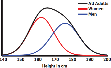
Figure 8.1: Height distribution for men, women and all adults.

But the above reasoning hinges on the existence of a fixed mixture distribution, which requires the mixture ratio of all those factors to be fixed. What justifies treating the gender mixture as fixed? What if we want to make inferences about subsets of the population that may have different gender ratios? When we consider the possibility that the gender ratio might not be fixed, we are implicitly talking about extending the results from the current dataset to a future dataset that might have a different gender ratio. That is, we want to know if treating the gender ratio as fixed will affect the external validity of inferences made from the current data.

In A/B tests, external validity often concerns bias resulting from differences between the population from which the inference was drawn and the population upon which the inference will be later applied. When extending externally, inferences can be made invalid due to an under-estimation of uncertainty. Imagine that we sample students from 2 of 20 local 7th grade classes at random to estimate the average height of all local 7th graders. We assume that the height distributions of boys and girls in the 20 schools are the same. If we also assume the gender ratios in the 20 schools are fixed, then we can assume heights of sampled students are i.i.d. from a single mixture distribution and form a confidence interval for the mean of height. But what if even though the gender ratio is close to 50/50 in the whole school district, there exist large differences in gender ratios at different schools? Then it is possible that the two randomly chosen schools have significantly more boys than girls, or vice versa. Under this scenario, the confidence interval we get by assuming a fixed gender ratio and i.i.d. heights will be too narrow because it does not account for the variability of gender ratios among the 20 schools. In other words, the gender ratio for a sample we got may not be “representative” for the general population we want our results to apply to. To make the result externally valid, we must treat gender ratio as a random variable.

The following simulation illustrates this point. Table 8.1 shows female and male student counts in 20 hypothetical schools. It is constructed such that:

1. Each school has exactly 1,000 student.
2. School #1 has 690 female and 310 male students. Each incremental school has 20 fewer females and 20 more males than the previous school. School #20 has 310 female and 690 male students.
   
3. In total, the gender ratio is balanced with exactly 10,000 female students and 10,000 male students.

Table 8.1: Female and male students configuration in a hypothetical 20 school district.

School	Female Count	Male Count
1	690	310
2	670	330
3	650	350
4	630	370
5	610	390
	\(\cdots\)	\(\cdots\)
15	410	590
16	390	610
17	370	630
18	350	650
19	330	670
20	310	690

We generate male heights from a normal distribution with mean 175cm and standard deviation 10cm. Female heights are generated from a normal distribution with mean 160cm and standard deviation 10cm. This simulated data is assumed to be the true heights for each of the 20,000 students. In this dataset, the true average height over the 20,000 students is 167.46. The goal is to sample 200 students out of the 20,000 students to estimate the average height.

Table 8.2 shows the results from the 4 sampling methods. In Case 1 we randomly sample 200 students from the combined 20,000 students. For Cases 2 to 4, we use a two-stage sampling. For Case 2 we first sample 2 schools from the 20 schools, and then sample 100 students from each of the 2 chosen schools. In cases 3 and 4 we sample 5 and 10 schools, then 40 students and 20 students for each chosen school, respectively. In all cases we sample 200 students. For each case, after we sampled 200 students, we compute the sample average and also standard deviation from the standard variance formula assuming i.i.d. observations. We used that to compute the 95% confidence interval and recorded whether the true average 167.46 was within the interval. We repeated this process 2,000 times and then compute the coverage, average estimated standard error from the standard formula, and standard deviation of the 2,000 sample averages (which approximates the true standard error of the mean).

Table 8.2 shows that case 1 has the correct coverage at 95% and the standard variance formula produces a standard error that is very close to the truth. In all other cases, coverages are all lower than the promised 95%, true standard errors are all larger than those given by standard formula, confirming variance under-estimation. In fact, in all cases the standard formula gives very similar standard errors. This is because it assumes i.i.d. sampled heights. However, when samples are from a small number of randomly selected schools, there is extra variation in the population due to the fluctuation of gender ratio, making the true standard error larger than under the i.i.d. assumption. We saw as the number of schools sampled in the first stage increased from 2 to 10, the true standard deviation decreased and coverage got better. In cases 2-4, if we assume sample observations are i.i.d. and use the standard variance formula, then the inference is only valid for the average height of the chosen schools and cannot be extended to all 20 schools. If we want to make the extended inference, we need to correctly account for additional “between school” variance.

Table 8.2: Comparison of 4 sampling mechanisms. The first is a random sample from all students; the other 3 cases select 2, 5 and 10 schools respectively and then sample students from the chosen schools. Results show that the standard variance formula (assuming i.i.d. observations) under-estimates the true variance and gives lower coverage than the promised 95% level.

Case	#School	Coverage	SE with standard formula	True SE
1	20	0.949	0.879	0.880
2	2	0.753	0.877	1.446
3	5	0.866	0.878	1.141
4	10	0.916	0.879	0.976

From both the numbers in an urn and estimating student’s height examples, we summarize the reasoning of independence (or lack thereof) in the following steps:

1. Sampling: We identify an unit from which we can randomly sample from.
2. Hierarchical Model and Conditional Independence: In reality, observations at the level of the sampling unit are often considered to be dependent on certain higher level factors (e.g. same gender, age, location for users) and many units share a similar value of those factors form clusters. Under this hierarchical model, conditioned on these factors, the sampling unit are independent within each cluster.
   
3. Factor Mixture and Independence: When the mixture of the factors (e.g. gender ratio, etc.) in the population is considered to be fixed and not varying. The whole distribution of the observations from the sampling unit can be modeled as independently drawn from a mixture distribution.
4. External Validity: Independence assumption relies on treating factor mixture as fixed and not varying. Therefore any results under the independence assumption is tied to the population with a particular mixture of the factors. These results cannot be extended to another population with a very different factor mixture.

Let us apply the steps to the unit of user — the commonly assumed unit of independence. Ignoring any practical user tracking issue and assuming we can always identify a user, we can certainly randomly sample users from the whole population of users. For any observation at user level, the higher level factors determining the distribution of such observations has a mixture for the population of users from which we sample from in a given period of time. When we treat this mixture as fixed, we can assume observations at user level to be i.i.d. What is the price to pay to treat the mixture as fixed? The price is we can only derive results for the specific set of user population and the specific period of time when we run the experiment. That is, external validity implies that results from today’s experiment to predict tomorrow’s behavior may not perfect, and results should always be interpreted within the tested population. If we want to allow the population mixture to change and need our results to incorporate this uncertainty, then we cannot assume users to be i.i.d. and our estimation of average treatment effect will have bigger variance and wider confidence intervals than the estimations when users are assumed to be i.i.d. There is no free lunch, the more uncertainties we want to include in our analyses, the less accuracy our estimation will be.

By connecting the i.i.d. assumption with external validity, we now understand that the i.i.d. assumption is ultimately not justified by theory, but by choice. In other words, we can make conscious choices to limit the external validity of the results we get, in exchange for independence assumption. This means the question of independence can often be flipped to be a question of external validity. We can apply this argument to units like users, groups or community of users, locations, devices and many other units to justify independence assumption. However, reasoning with external validity may be very subtle in some cases and deemed a bit subjective. For example, if we randomly sample page-views, what is the factor mixture and what does it mean to external validity by fixing this mixture? In practice, many A/B testing practitioners uses the following rule of thumb:

Observations at the level of the randomization unit can be treated as independent.

We call this randomization unit principle (RUP). The most common randomization unit is user, and we just applied the external validity argument to justify treating it as independent unit. But we have ignored the issues of user tracking. When user tracking uses cookie, we know the real same user can appear as multiple “users.” Other popular randomization units include visit/session, page-view/impression. These units are all more granular than user. In the next section, we will justify RUP from a different angle by showing the following result.

For any randomization unit more granular than an independent unit, we can approximately compute the variance of the ATE estimator assuming randomization unit is independent.

This result means RUP for variance estimation only relies on the existence of an independent unit less granular than the randomization unit. That is, we do not necessarily need to wrestle with external validity for independence assumption of the randomization unit itself, we only need to assume some independent unit exists above the randomization unit!

8.4.2 Variance Estimation for Average and Weighted Average

Variance estimation is directly impacted by the data generating process and independence assumption. If the metric is an average of \(Y_i,i=1,\dots, N\), the variance of the metric is \(\mathrm{Var}(Y)/N\) only when \(Y_i\) are independent. Using the variance formula for the independent case to cases where observations are not independent often lead to wild miss-estimation of the variance and invalidate the whole analysis.

We already introduced the three different units:

1. \(\mathcal{I}\): the Independent unit.
2. \(\mathcal{R}\): the randomization unit.
3. \(\mathcal{A}\): the analysis unit.

We posit the existence of an independent unit \(\mathcal{I}\). In the previous section we explained the justification of independence is deeply connected with external validity and we argued units like user can usually be treated as independent unit.

Randomization unit \(\mathcal{R}\) is the unit we use to randomize. When \(\mathcal{R}\) is less granular than \(\mathcal{I}\) (randomization units are clusters of \(\mathcal{I}\) and the clustering is random), the randomization unit is itself an independent unit. Therefore, only three cases are relevant:

1. \(\mathcal{I} = \mathcal{R} = \mathcal{A}\)
2. \(\mathcal{I} = \mathcal{R} > \mathcal{A}\)
3. \(\mathcal{I} > \mathcal{R} \ge \mathcal{A}\)

We provide variance estimations for the ATE estimator \(\Delta =M_t - M_c\) for all the three cases.

Case 1: \(\mathcal{I} = \mathcal{R} = \mathcal{A}\). Consider metrics defined as an average. Since the analysis unit is also an independent unit, both the treatment and control metric \(M_t\) and \(M_c\) are average of independent observations \(Y_i\). Also, as the randomization unit is also the independent unit, the two metric values \(M_t\) and \(M_c\) are independent because treatment and control groups are independent. We have,

\[\begin{align*} \mathrm{Var}_\text{S}(\Delta) & = \mathrm{Var}(\overline{Y^{t}})+ \mathrm{Var}(\overline{Y^{c}}) \\ & = \frac{\sigma_t^2}{n_t} + \frac{\sigma_c^2}{n_c}, \end{align*}\] where the subscript \(S\) means the “simple” case, \(\sigma_t^2\) and \(\sigma_c^2\) are variance of the independent observations \(Y_i\) for treatment and control groups respectively, and \(n_t\) and \(n_c\) are count of the observations.

\(\sigma_t^2\) and \(\sigma_c^2\) are to be estimated using sample variance formula \[ \widehat{\sigma_g}^2 = \frac{\sum_i (Y^{(g)}_i - \overline{Y^{(g)}})^2}{N_g-1},\quad g = t,c\,. \]

Consider metrics defined as weighted average. Let \(w_i\) be the weight for the i-th observation. The treatment metric has the form \[ M_t = \frac{\sum_i w_i^{(t)} Y^{(t)}_i}{\sum_i w_i^{(t)}}\,. \]

This is a ratio of two sums, which also have an asymptotic normal distribution thanks to the delta method (Casella and Berger 2002; Alex Deng, Knoblich, and Lu 2018). The variance of \(\Delta\) is \[\begin{align*} \mathrm{Var}_\text{D}(\Delta) & = \mathrm{Var}\left (\frac{\sum_i w_i^{(t)} Y^{(t)}_i}{\sum_i w_i^{(t)}}\right) + \mathrm{Var}\left(\frac{\sum_i w_i^{(c)} Y^{(c)}_i}{\sum_i w_i^{(c)}}\right)\\ & = \frac{\xi_t^2}{n_t} + \frac{\xi_c^2}{n_c} \end{align*}\] where the subscript \(D\) means delta method was used, \(\xi_t^2\) and \(\xi_c^2\) are the delta method variance. To estimate the two delta method variance, let \(S_i^{(g)} = w_i\cdot Y_i^{(g)}\) for both groups \(g=t,c\). \[\begin{equation} \xi_g^2 = \frac{1}{\mathrm{E}(w^{(g)})^2}\mathrm{Var}(S^{(g)}) + \frac{\mathrm{E}(S^{(g)})^2}{\mathrm{E}(w^{(g)})^4}\mathrm{Var}(w^{(g)})\\ - 2 \frac{\mathrm{E}(S^{(g)})}{\mathrm{E}(w^{(g)})^3} \mathrm{Cov}(S^{(g)},w^{(g)})\,,\quad g=t,c \tag{8.2} \end{equation}\] where all the expectations, variances and covariance can be estimated using sample mean, sample variance and sample covariance. The details of the delta method is included in the appendix 11.2. See Alex Deng, Knoblich, and Lu (2018) for more applications of the delta method in A/B testing.

Case 2: \(\mathcal{I} = \mathcal{R} > \mathcal{A}\). When the analysis unit \(\mathcal{A}\) is more granular than the independent and randomization unit \(\mathcal{R}\), the observations \(Y_i\) and weights \(w_i\) are not independent anymore. We need to modify the notation a little. We will keep using \(i\) as the index for independent (and in this case randomization) unit, and use \(j\) to index the observations at the analysis unit level. Observations are now denoted as \(Y_{ij}^{g}, i = 1,\dots,n_g, j = 1,\dots,N_i^{g}, g = t,c\). Also let \(N_g = \sum_i N_i^{(g)}\) to be the total count of analysis unit for each group.

Using a concrete example, if randomization unit is user and analysis unit is page-view. \(Y_{ij}^{(g)}\) is the j-th page-view level observation for the i-th user, \(n_g\) is the number of users, and \(N_g\) is the number of page-views.

Average metrics have the form \[ \overline{Y^{(g)}} = \frac{\sum_i \sum_j Y_{ij}^{(g)}}{\sum_i N_i^{(g)}}\,. \] Let \(S_i^{(g)} = \sum_j Y_{ij}^{(g)}\), \[ \overline{Y^{(g)}} = \frac{\sum_i S_i^{(g)}}{\sum_i N_i^{(g)}}\,. \] This is again a ratio of sum of independent unit level observations — the same form we have seen in Case 1 for weighted average.

We show the weighted average for this case also have a similar form. Let \(w_{ij}^{(g)}\) be the weight and \[ \overline{Y^{(g)}} = \frac{\sum_i \sum_j w_{ij}^{(g)}Y_{ij}^{(g)}}{\sum_i \sum_j w_{ij}^{(g)}} = = \frac{\sum_i S_i^{(g)}}{\sum_i W_i^{(g)}}\,. \] where \(S_i^{(g)} = \sum_j W_{ij}^{(g)}Y_{ij}^{(g)}\), \(W_i^{g} = \sum_j w_{ij}^{(g)}\).

Therefore, for both average and weighted average metrics, they can be expressed as a ratio of sum of i.i.d. observations (at the independent unit level). Their variance can be estimated using the delta method similar to Equation (8.2).

Case 3: \(\mathcal{I} > \mathcal{R} \ge \mathcal{A}\). This is the most complicated case, as the same independent unit can be further split between the treatment and control group. We will use i to index independent unit, and j to index the randomization unit. In Case 2, we saw that both average and weighted average metrics have the same form \[ \widehat{Y^{(g)}} = \frac{\sum_i S_i^{(g)}}{\sum_i W_i^{(g)}}\,, \] where \(S_i^{(g)}\) and \(W_i^{(g)}\) are both observations at the randomization unit level, and both have a form as a sum of analysis unit level observations.

Unlike Case 2 where observations \((S_i^{(g)}, W_i^{(g)})\) for treatment group and control group are independent, and we can apply the delta method to the two groups separately and then add the two estimated variance up to get the estimated variance for the \(\Delta\). In Case 3 the same independent unit contains observations in both groups so there is dependency between the treatment and control groups!

Let \((S_i^{(t)}, W_i^{(t)},S_i^{(c)}, W_i^{(c)}),i=1,\dots,n\) be independent observation vectors, the ATE estimator is \[ \Delta = \frac{\sum_i S_i^{(t)}}{\sum_i W_i^{(t)}} - \frac{\sum_i S_i^{(c)}}{\sum_i W_i^{(c)}}\,. \] The multivariate version of the central limit theorem says the sample mean of the 4-d vector \((S_i^{(t)}, W_i^{(t)},S_i^{(c)}, W_i^{(c)}),i=1,\dots,n\) converge in distribution to a multivariate normal distribution. Since \(\Delta\) is a continuous function of the sums (or sample mean) of \((S_i^{(t)}, W_i^{(t)},S_i^{(c)}, W_i^{(c)})\), we can again apply the delta method to get a formula for \(\mathrm{Var}_{\text{G}}(\Delta)\), where the subscript G stands for “general” since Case 3 is the most general case as this formula contains the other two cases as special cases.

The delta method can also be interpreted as the following. Asymptotically, \(\sqrt{n}(\Delta - \delta)\) has the same normal distribution as the average of \[\begin{equation} \frac{{S_{i}^{(t)} - W_{i}^{(t)}\cdot \mu_t}}{p \mu_w} - \frac{{S_{i}^{(c)} - W_{i}^{(c)} \cdot \mu_c}}{(1 - p)\mu_w}\,,i=1,\dots,n\,, \tag{8.3} \end{equation}\] where \[ \mu_t = \frac{\mathrm{E}(S^{(t)})}{\mathrm{E}(W^{(t)})}\,,\mu_c = \frac{\mathrm{E}(S^{(c)})}{\mathrm{E}(W^{(c)})}\,,\\ \mu_w = \mathrm{E}(W^{(t)}+W^{(c)}) \] can all be estimated accordingly, and \(p\) is the randomization probability for the treatment group. This is an average of i.i.d. random variables and its variance can be estimated using sample variance formula.

Using the the general variance formula, Alex Deng, Lu, and Litz (2017) studied the difference between the general variance formula result, to the RUP results where \(\mathcal{R}\) is assumed to also be independent. Note that if we assume \(\mathcal{R}\) to be an independent level, then there is no dependency between the two groups, which simplifies the variance estimation quite a lot. Here are a summary of their key results.

1. The RUP results and the general formula are not exactly the same. RUP may under-estimate the variance.
2. The difference is 0 when the treatment effect at each independent unit level, defined as \(\tau_i = E(Y_{ij}^{(t)})\)-\(E(Y_{ij}^{(c)})\) is a constant. That is, when all individual treatment effects are the same and there is no treatment effect heterogeneity, RUP agrees with the general formula. Note that this is also true under the sharp null hypothesis that there is no treatment effect for every independent unit.
3. The under-estimation of the standard error by RUP is the same order of the treatment effect. When the treatment effect is small, the under-estimation is also small.

This result gives us another way to justify RUP. When the effect is large, because of large sample sizes in A/B tests, inferences are robust against underestimation of the variance. In fact, a percent effect more than 5% is considered a large effect in A/B testing. But a 5% underestimation of the standard error has a much smaller impact to the trustworthiness of the inference comparing to the caveat of external validity. The practical implication of this result is that we only need to posit the existence of an independent unit for which the induced external validity implication are acceptable, and any randomization unit equal or more granular than that independent unit can practically be treated also as independent for the purpose of variance computation.

Another application of the general variance formula for Case 3 is for cases where the randomization unit are not recorded properly or intentionally removed from the data. Why do we want to remove the randomization unit info from the data? For privacy! Sometimes it is required that the data needs to be anonymized so that we cannot identify a user from the data and map a user’s strong identifier such as user name or email address by a pseudo random GUID is not enough and we have to mix multiple users into the same GUID so that it is impossible to differentiate users with the same GUID apart. When doing so, this new GUID can be treated as independent unit and all we need to apply the general variance formula (for example, see Equation (8.3)) is to be able to compute \((S_i^{(t)}, W_i^{(t)},S_i^{(c)}, W_i^{(c)}),i=1,\dots,n\) for each independent unit. That is, we can still perform statistical analysis without the user identifier in the data to preserve anonymity.

Clustered Randomization. Case 2 \(\mathcal{I} = \mathcal{R} > \mathcal{A}\) is also referred to as clustered randomization. We first introduced clustered randomization in Section 3.3. Because analysis units are not sampled individually, but grouped by clusters, the variance of metrics will be larger than Case 1 where randomization unit is the analysis unit. Fail to correctly apply the delta method to estimate the variance results in underestimation of the variance and larger real false positive rate (Type I error) than the nominal significance level.

Under strict assumptions, closed-form variance formula for a sample average \(\overline{Y}\) with clustered randomization exists (Donner 1987; Klar and Donner 2001). For example, when the number of observations in each cluster \(N_i = m\) are all the same and the conditional variance of observations within each cluster \(\sigma_i^2 = \sigma^2\) are also the same for all \(i,\) \[\begin{equation} \mathrm{Var}(\bar{Y}) = \frac{\sigma^2+\tau^2}{nm}\{1+(m-1)\rho\}, \tag{8.4} \end{equation}\] where \(\tau^2 = \mathrm{Var}(\mu_i)\) is the variance and \(\rho = \tau^2 / (\sigma^2+\tau^2)\) is the coefficient of intra-cluster correlation, which quantifies the contribution of between-cluster variance to the total variance. To facilitate understanding of the variance formula , two extreme cases are worth mentioning:

1. If \(\sigma=0,\) then for each \(i=1,\dots,K\) and all \(j = 1, \ldots, N_i,\) \(Y_{ij} = \mu_i.\) In this case, \(\rho=1\) and \(\mathrm{Var}(\overline{Y})=\tau^2/K;\)
2. If \(\tau=0\), then \(\mu_i = \mu\) for all \(i=1, \ldots, K,\) and therefore the observations \(Y_{ij}\)’s are in fact i.i.d. In this case, \(\rho=0\) and Equation (8.4) reduces to \(\mathrm{Var}(\overline{Y})=\sigma^2/(nm) = \sigma^2/N\).

Unlike the delta method variance estimator Equation (8.2), Equation has only limited practical value because the assumptions it makes are unrealistic. In reality, the cluster sizes \(N_i\) and distributions of \(Y_{ij}\) for each cluster \(i\) are different, which means that \(\mu_i\) and \(\sigma_i^2\) are different. But it did illustrate that the coefficient of intra-cluster correlation is one of the reason why clustered randomization has larger variance.

If we look closer to the delta method variance Equation (8.2), the second term is \[ \frac{\mathrm{E}(S^{(g)})^2}{\mathrm{E}(w^{(g)})^4}\mathrm{Var}(w^{(g)}) \] where \(\mathrm{E}(w^{(g)})\) and \(\mathrm{Var}(w^{(g)})\) are the mean and variance of the total weights in a cluster. For simple average total weights for the i-th cluster is just \(N_i\) — the number of analysis units within each cluster. Equation (8.2) tells us not only the coefficient of intra-cluster correlation plays a role, but also the variance of the cluster size! To reduce variance of the metric, clusters with more homogeneous sizes are preferred to clusters with very different sizes.

Another common approach to study clustered randomization is to use a mixed effect model, also known as multi-level/hierarchical regression (Gelman and Hill 2006). In a such model, we model the observations at analysis unit level \(Y_{ij}\) to be conditionally independent with mean and variance \(\mu_i\) and \(\sigma_i^2\) for each cluster, while the parameters themselves follow a higher order distribution represents heterogeneity of clusters. Under this setting, we can infer the treatment effect as the “fixed” effect for the treatment indicator term¹⁹. Stan (Carpenter et al. 2016) implements a Markov Chain Monte Carlo (MCMC) solution to infer the posterior distribution of those parameters, but this needs significant computational effort when data is big. Moreover, the estimated ATE, i.e., the coefficient for the treatment assignment indicator, is for the randomization unit (i.e., cluster) but not the analysis unit level, because it treats all clusters with equal weights and can be viewed as similar to the double average \(\sum_i (\sum_j Y_{ij} / N_j) / n,\) which is usually different than the population average \(\overline Y\) (A. Deng and Shi 2016). This distinction doesn’t make a systematic difference when effects across clusters are homogeneous. However, in reality the treatment effects are often heterogeneous, and using mixed effect model estimates without further adjustment steps could lead to biases. Proper reweighting adjustment does exists (Alex Deng, Knoblich, and Lu 2018).

8.5 Central Limit Theorem and Normal Approximation

So far we have been assuming the sampling distribution of a metric \(M\), being either average, weighted average or percentile, can be approximated by a normal distribution once the sample size (of independent observations) is large enough. This is from the central limit theorem (CLT), which says for i.i.d. random variables \(X_i,i=1,\dots,n\) with mean \(\mu\) and finite variance \(\sigma^2\), \[ \sqrt{n} \left( \overline{X} - \mu \right) \xrightarrow{d} \text{Normal}(0,\sigma^2) \,, \] where the convergence is in the sense of convergence in distribution (Van der Vaart 2000). When \(X\) has vector value, such as in the weighted average and clustered randomization case where \(\mathcal{R}>\mathcal{A}\), the multivariate version of CLT \[ \sqrt{n} \left( \overline{X} - \mu \right) \xrightarrow{d} \text{Normal}(0,\Sigma) \,, \] is used, where \(\mu\) is the mean vector and \(\Sigma\) is the covariance matrix.

To apply the classic CLT, we need both i.i.d. and finite variance. Finite variance can be usually justified because most observations used to define metrics are naturally bounded. For potentially unbounded metrics, such as time-to-click, in practice we will always cap it (winsorize) by a practical bound. This will both gives us finite variance, and also crucial to tame the variance of the metric so it can achieve a reasonable statistical power. For the i.i.d. assumption, we justified it by connecting it to external validity and the randomization unit principle.

However, being an asymptotic result, CLT does not tell us how fast is the convergence to normal distribution and how large of sample size is needed.

The answer to this question varies. One rule of thumb and widely adopted opinion is normal approximation works for \(n>30\). This seems to be easily achievable in A/B tests where sample sizes are typically at least in thousands. In this section, we will look closer and suggest a required sample size to be at the order of \(100s^2\), where \[ s = \frac{\mathrm{E}((X-\mu)^3)}{\sigma^3} \] is the skewness of \(X\).

The key to study the convergence to normal is to use Edgeworth series (Hall 2013) that further explore the residual terms beyond the normal approximation. Let \(F(x)\) be the cumulative distribution function of \(\sqrt{n} ( \overline{X} - \mu )/\sigma\) and \(\Phi(x)\) and \(\phi(x)\) be the cumulative distribution function and density function for the standard normal. Boos and Hughes-Oliver (2000) showed that
\[\begin{equation} F(x) = \Phi(x) - \frac{6}{\sqrt{n}}s(x^2 - 1)\phi(x)+ O(1/n) \tag{8.5} \end{equation}\]

Three comments:

1. The first error term involves the skewness s and is in the order of \(n^{-1/2}\).
2. The second error term is in the order of \(1/n\) and the constant term not shown above actually involves the 4th standardized moment kurtosis as well as skewness.
3. If skewness is 0, e.g. when \(X\) is symmetric, converge to normal increases from \(1/\sqrt{n}\) to \(1/n\) — an order of \(n^{1/2}\) faster.

Let us focus on the first error term \(\frac{6}{\sqrt{n}}s(x^2 - 1)\phi(x)\). For a typical 95% two-sided confidence interval, we look at the 2.5% and 97.5% percentile, and they are very close to -1.96 and 1.96 for the standard normal distribution. Let \(x = \pm 1.96\) and if we want this error term to be less than 0.25%, then we will be getting \(n > 122.56s^2\). For a true 95% confidence interval, the probability of missing the true mean at the right and at the left are both 2.5%. With \(n > 122.56s^2\) independent samples, ignoring higher order error terms, the actual probability of missing the true mean at the right and left are below 2.75%. That is, we need a sample size of the order of \(100s^2\) if we want true missing out rate to be within 10% of the designed level. Boos and Hughes-Oliver (2000) also showed error term for a t-statistic when the variance is unknown. It is similar to the know variance case and they only differ by a constant term and error is bigger due to the unknown variance. Kohavi et al. (2014) derived \(355s^2\) based on similar calculation for the unknown variance case. Overall we think the order of \(100s^2\) is a better rule of thumb than \(n>30\).

Most metrics don’t have a large skewness more than 5, and the required sample size is less than 2,500. Kohavi et al. (2014) reported revenue per user to have a skewness of 17.9 from one of their dataset, and more than 30,000 sample size to get to the desired error limit based on our \(100s^2\) rule. However, once a proper capping was applied, that is to apply the function \(f(x) = min(x,c)\) for a cap c, the skewness dropped to 5 and the required sample size dropped to 2,500!

Surprisingly, the most common example of high skewness metric does not even involve large metric value. In fact, a Bernoulli distribution with \(p\) close to either 0 or 1 can have huge skewness. If we have a metric that tracks occurrence of certain rare events, such as client error rate. The metric itself is average of binary observations and the skewness of a Bernoulli(\(p\)) distribution is \(\frac{1-2p}{pq}\) where \(q=1-p\). When \(p\) is close to 0, this is about \(1/\sqrt{p}\). A (not so rare) event with \(p\) around \(10^{-4}\) can lead to a skewness of 100!

Figure 8.2 show the sampling distribution of a mean of 50,000 i.i.d. Bernoulli random variables with p=\(10^{-4}\). Our recommended sample would be \(10^6\) and 50,000 is still very much short of that. As expected, the distribution is far from normal and right-skewed, as easily seen from the QQ plot. We also observed that the distribution is still very discrete, because \(np\) in this case is only about 5.

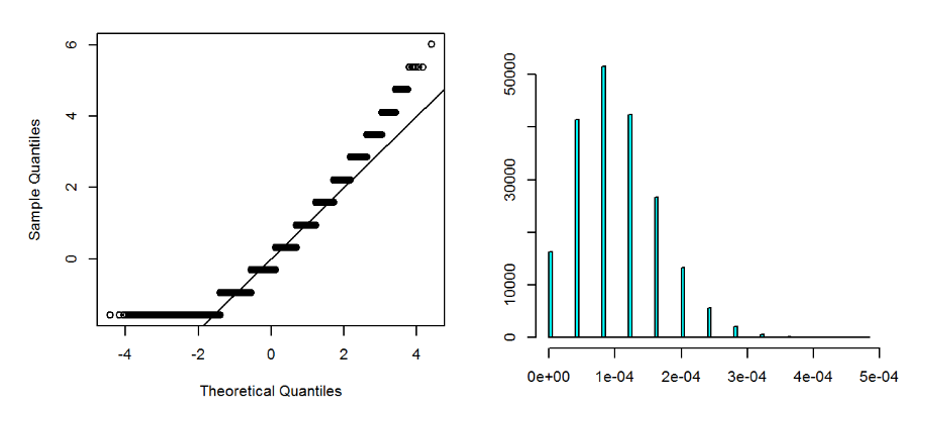
Figure 8.2: Right: Sampling distribution of sample mean of 50,000 i.i.d. Bernoulli random variables with p=\(10^{-4}\). Left: QQ-Norm plot. Right: Histogram. The distribution is discrete and severely right-skewed.

What should we do in cases like this? There are two approaches. The practical approach is to use a balanced design where treatment and control are of the same sample size. The alternative is to adjust the confidence interval or approximate the cumulative distribution function directly using Equation (8.5) with the error term. We focus on balanced design first and will introduce two simple adjustment methods for the Bernoulli case.

The reason balanced design mitigates the issue and require much less sample size for normal approximation to work is because we will be looking at the confidence interval of the ATE estimator \(\Delta\). When the sample size of treatment and control groups are exactly the same, \(\Delta\) is sample average of i.i.d. random variable \(Z = X - Y\) where X and Y are the random variable for observations in treatment group and control group respectively. The rationale is the skewness of \(Z\) is much smaller than \(X-Y\). In the sharp null hypothesis case where there is no individual treatment effect, X and Y have the same distribution and X-Y is symmetric with 0 skewness! When skewness is 0, the convergence to normal is \(\sqrt{n}\) faster, roughly meaning the sample size needed is square root of the sample size needed when skewness is the leading term. But even when skewness of Z is not exactly 0, reducing it by a factor of 10 reduces the sample size needed by a factor of 100! Figure 8.3 shows the sampling distribution for \(\Delta\) of two sample means of 50,000 i.i.d. Bernoulli random variables with p=\(10^{-4}\). This time we saw the distribution is much closer to normal, with only a little fatter tail. Figure 8.4 shows if the sample size is imbalanced, then the one with larger sample size will be closer to normal (90,000 samples in the example, close to 100,000 needed by \(100s^2\) rule) and the one with less sample size still shows strong skewness and discrete spikes, therefore \(\Delta\) behaves like mixture of many normal distribution with many modes. Because balanced design is often also optimal for the best statistical power, the normal approximation sample size requirement gives another reason to use a balanced design for high skewness metrics.

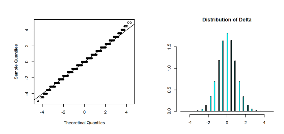
Figure 8.3: Right: Sampling distribution of the difference of two sample mean of 50,000 i.i.d. Bernoulli random variables with p=\(10^{-4}\). Left: QQ-Norm plot. Right: Histogram. The distribution of the difference is much closer to normal even though each sample mean is severely skewed.

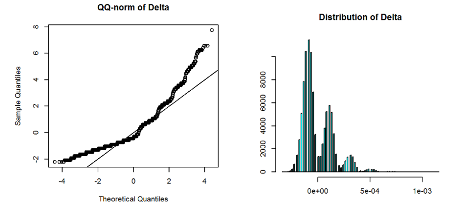
Figure 8.4: Right: Sampling distribution of the difference of two sample means of Bernoulli random variables with p=\(10^{-4}\), one with 10,000 i.i.d. sample and the other with 90,000. Left: QQ-Norm plot. Right: Histogram. The distribution is multi-model as a mixture of normal distributions.

The adjustment of confidence interval using Edgeworth expansion is known as the Cornish–Fisher expansion (S. R. A. Fisher and Cornish 1960). Also see Hall (2013). We found for high skewness due to large value, capping is the most effective and also improve statistical power. For Bernoulli rare event case, we introduce two simple and easy to implement adjustment methods. Both methods still use normal approximation but correct both the sample mean and the estimated variance. In both methods the derived confidence interval will have wider range and closer to the nominal coverage.

Let the total sample size be \(n\) and the sum of i.i.d. Bernoulli random variables \(n_1\). For small p \(n_1\) is small. The first adjustment is Laplace Smoothing, which artificially add one positive binary outcome to the Bernoulli samples. With this adjustment, the “sample mean” becomes \((n_1+1)/(n+1)\) and the estimated variance will also use the new adjusted “sample mean.”

The second adjustment is proposed in Agresti and Coull (1998) and known as Agresti-Coull correction. Like Laplace smoothing, it adds artificial observations to the samples. For two-sided confidence interval of \(1-\alpha\), let \(z_{\alpha/2}\) be the \(1-\alpha/2\) percentile of standard normal, Agresti-Coull adds \(z_{\alpha/2}^2\) artificial samples with half of them positive. The new “sample mean” becomes \(\tilde{p} = \frac{n_1+z_{\alpha/2}^2/2}{n+z_{\alpha/2}^2}\), and the variance of the approximate normal distribution for the sample mean is \(\frac{\tilde{p}(1-\tilde{p})}{n+z_{\alpha/2}^2}\). For 95% confidence interval, \(z_{\alpha/2}\) is about 2 and the adjustment is to simply add 4 instances with 2 successes.

8.6 Confidence Interval and Variance Estimation for Percentile metrics

Percentile (also called quantiles) metrics are widely used to focus on tails of distributions. This is very common for performance measurements, where we not only care about an average user’s experience, but even more care about those who suffer from the slowest responses. Within the web performance community, percentiles (of, for example, page loading time) at 75%, 95% or 99% often take the spotlight. In addition, the 50% quantile (median) is sometimes used to replace the mean, because it is more robust to outlier observations (e.g., due to errors in instrumentation and telemetry). This section focuses on estimating the variances of percentile metrics.

Suppose we have \(n\) i.i.d. observations \(Y_1,\dots,Y_n,\) generated by a cumulative distribution function \(F(Y) = P(Y\le y)\) and a density function \(f(y)\)²⁰. The theoretical p-th percentile for the distribution \(F\) is defined as \(F^{-1}(p)\). Let \(Y_{(1)}, \dots, Y_{(n)}\) be the ascending ordering of the original observations. The sample percentile at \(p\) is \(Y_{(np)}\) if \(np\) is an integer. Otherwise, let \(\lfloor np\rfloor\) be the floor of \(np\), then the sample quantile can be defined as any number between \(Y_{(\lfloor np\rfloor)}\) and \(Y_{(\lfloor np\rfloor +1)}\) or a linear interpolation of the two²¹. For simplicity here we use \(Y_{(\lfloor np\rfloor)},\) which will not affect any asymptotic results when \(n\) is sufficiently large. It is a well-known fact that, if \(Y_1, \ldots, Y_n\) are i.i.d. observations, following the central limit theorem and a rather straightforward application of the Delta method, the sample percentile is approximately normal (Casella and Berger 2002; Van der Vaart 2000): \[\begin{equation} \sqrt{n} \left\{ Y_{\lfloor np\rfloor} - F^{-1}(p) \right\} \xrightarrow{d} N \left[ 0, \frac{\sigma^2}{f \left\{F^{-1}(p)\right\}^2} \right], \tag{8.6} \end{equation}\] where \(\sigma^2 = p(1-p).\) However, unfortunately, in practice we may not have i.i.d. observations when randomization unit is not the same as the analysis unit. For site performance, randomizations are usually on users or devices but analysis unit are at each page-view/impression level.

Let \(I_i = I \{ Y_i \le F^{-1}(p) \},\) where \(I\) is the indicator function. The proof of Equation (8.6) involves a key step to compute \(\mathrm{Var}(\overline I)\).²² When \(Y_i\) are not independent, we use the delta method to compute \(\mathrm{Var}(\overline I)\) and the only change in the result would be to replace \(\sigma^2 = p(1-p)\) by the adjusted standard deviation. That is, Equation (8.6) still holds in the clustered case with \(\sigma^2 = n \mathrm{Var}(\overline I)\). This generalizes the i.i.d. case where \(n\mathrm{Var}(\overline I) = p(1-p)\).

It is still difficult to apply Equation (8.6) in practice because the denominator \(f \{ F^{-1}(p) \}\) involves the unknown density function \(f\) at the unknown true quantile \(F^{-1}(p).\) A straightforward approach is to estimate \(f\) from the observed \(Y_i\) using non-parametric methods such as kernel density estimation (Wasserman 2003). However, any non-parametric density estimation method is trading off between bias and variance. To reduce variance, more aggressive smoothing and hence larger bias need to be introduced to the procedure. This issue is less critical for quantiles at the body of the distribution, e.g. median, where density is high and more data exists around the quantile to make the variance smaller. As we move to the tail, e.g. 90%, 95% or 99%, the noise of the density estimation gets bigger, so we have to introduce more smoothing and more bias. Because the density shows up in the denominator and density in the tail often decays to \(0\), a small bias in estimated density can lead to a big bias for the estimated variance (Brown and Wolfe (1983) raised similar criticisms with their simulation study). A second approach is to bootstrap, re-sampling the whole dataset many times and computing quantiles repeatedly. Unlike an average, computing quantiles requires sorting, and sorting in distributed systems (data is distributed in the network) requires data shuffling between nodes, which incurs costly network I/O. Thus, bootstrap works well for small scale data but tends to be too expensive in large scale in its original form (efficient bootstrap on massive data is a research area of its own (Kleiner et al. 2014)).

Alex Deng, Knoblich, and Lu (2018) introduced a novel idea to estimate percentile variance without estimating the unknown density function. Recall that \(I_i = I \{Y_i \le F^{-1}(p) \}\). \(\sum I_i\) is the count of observations no greater than the quantile. Consider the independent case where \(I_i\) are i.i.d., \(\sum I_i\) follows a binomial distribution. Consequently, when \(n\) is large \(\sqrt{n}(\overline I-p) \approx \text{Normal}(0, \sigma^2)\) where \(\sigma^2 = p(1-p)\). If the quantile value \(F^{-1}(p) \in [Y_{(r)},Y_{(r+1)}),\) then \(\overline I = r/n\). The above equation can be inverted into a \(100(1-\alpha)\%\) confidence interval for \(r/n:\) \(p \pm z_{\alpha/2}\sigma/\sqrt{n}\). This means with 95% probability the true percentile is between the lower rank \(L = n(p-z_{\alpha/2}\sigma/\sqrt{n})\) and upper rank \(U = n(p+z_{\alpha/2}\sigma/\sqrt{n})+1\)! Now consider the general case where \(I_i\) are not independent. \(\sum I_i\) would not follow a binomial distribution but the central limit theorem stills applies and the variance of \(\overline{I}\) can be estimated using the delta method. The above procedure still works with a small adjustment to make: we can no longer assume \(\sigma^2 = p(1-p)\) as in the independent case and instead need to do an extra step of delta method to estimate \(\sigma^2\).

To summarize, the confidence interval for a percentile can be computed in the following steps:

1. Fetch the quantile \(Y_{(\lfloor np\rfloor)}\).
2. Compute \(I_i = I \{Y_i \le Y_{(\lfloor np\rfloor)}\)}.
3. Apply the delta method to estimate \(\mathrm{Var}(\overline{I})\).
4. Compute \(\sigma\) by setting \(\sigma^2/n\) equal to the estimated variance of \(\overline{I}\).
5. Compute \(L,U = n(p \pm z_{\alpha/2}\sigma)\).
6. Fetch the two ranks \(X_{(L)}\) and \(X_{(U)}\).

We call this percentile CI with pre-adjustment²³. This method reduces the complexity of computing a percentile and its confidence interval into a Delta method step and subsequently fetching three “ntiles.” Alex Deng, Knoblich, and Lu (2018) also proposed a slightly different percentile CI with post-adjustment method that has some computational advantages over the pre-adjustment method:

1. Compute \(L,U = n(p \pm z_{\alpha/2}\sqrt{p(1-p)/n})\).
2. Fetch \(Y_{(\lfloor np\rfloor)}\), \(Y_{(L)}\) and \(Y_{(U)}\).
3. Compute \(I_i = I \{Y_i \le Y_{(\lfloor np\rfloor)}\)}.
4. Apply the delta method to estimate \(\mathrm{Var}(\overline{I})\).
5. Compute \(\sigma\) by setting \(\sigma^2/n\) equal to the estimated variance of \(\overline{I}\).
6. Compute the (multiplicative) correction factor \(\sigma / \sqrt{p(1-p)}\) and apply it to \(X_{(L)}\) and \(X_{(U)}\).

The post-adjustment method computes the percentile CI pretending \(Y\) to be independent. Because Equation (8.6) tell us the only change we need to make from independent to clustered randomization case is to adjust the variance of the asymptotic normal distribution by a rescale factor of \(\frac{\sigma^2}{p(1-p)}\), the confidence interval should also be adjusted accordingly by a rescale of \(\frac{\sigma}{\sqrt{p(1-p)}}\)!

Using CLT and assuming sample percentile is approximately normally distributed, we can then convert any \(1-\alpha\) two-sided confidence interval to the variance of sample percentile. Note that confidence interval from the percentile CI method might not be exactly symmetric. In practice we can make it symmetric by picking the larger width of the two sides as the half width of a symmetric interval.

8.7 p-Value, Statistical Power, S and M Error

The whole large sample theory of A/B testing²⁴ for ATE is based on the asymptotic normality of \(\Delta\), \[ \frac{\Delta - \delta}{\sqrt{\sigma_t^2/n_t + \sigma_c^2/n_c}} \xrightarrow{d} \text{Normal}(0,1)\,. \] We spent a few sections in this chapter digesting components of this result: the independent assumptions, the sample size needed for the normal approximation and variance estimation — all are critical to ensure trustworthy inferences. In this section we use it to summarize results and interpret them.

8.7.1 p-Value

Let \(Z = \frac{\Delta}{\sqrt{\sigma_t^2/n_t + \sigma_c^2/n_c}}\) be the observed z-score. Given a pre-specified Type I error bound \(\alpha\), we can derive the two-sided rejection region to be \(|Z| > z_{\alpha/2}\). This is because under null hypothesis \(\delta=0\), \(Z\) follows a standard normal distribution. Let \(\mathcal{Z}\) be the standard normal random variable, \[ P(|Z| \ge z_{\alpha/2}|H_0) = P(|\mathcal{Z}|\ge z_{\alpha/2}) = \alpha\,. \] We say this rejection region controls the Type I error, also called false rejection or false positive rate.

Rejection by a pre-specified Type I error bound and the corresponding rejection region is a binary decision. In practice, people prefer to use a continuous quantity. One choice is to just use the observed Z-score. A more common approach is to map Z-score to p-value defined as \[ P(|\mathcal{Z}|\ge|Z|)\,. \] Here the observed Z-score \(Z\) was considered to be fixed and p-value represents the probability that under the null hypothesis we will get a Z-score (absolute value in two-sided test case) more extreme than or equal to the observed one. p-value is always between 0 and 1 and p-value of \(\alpha\) corresponds to a Z-score of \(z_{\alpha/2}\).

p-value is more popular than Z-score because it has the scale of a probability and it has a probabilistic meaning. For Type I error bound of \(\alpha\), the rejection region can be defined simply for all p-values less than \(\alpha\). For a given experiment, the smaller a p-value is, the stronger the evidence against the null hypothesis based on the observations we got. However, the probabilistic nature and the seemingly simple definition makes p-value notoriously easy to be misinterpreted! Goodman (2008) documented 12 common misunderstandings. We summarize two patterns here.

Misunderstanding 1. A p-value of 5% means the null hypothesis has only a 5% chance of being true.

This statement is false because p-value does not tell us the probability of null hypothesis being true. The definition of p-value is a conditional probability of observing certain statistic given the null hypothesis is true. Roughly speaking, it is similar to \(P(Data|H_0)\). (\(P(Data|H_0)\) is the likelihood of observing the data under the null hypothesis. This is different from the probability of observing a z-score beyond the observed one. But they represents similar idea in the current context.) This is very different from \(P(H_0|Data)\), which is the probability the null hypothesis being true given what have been observed. In an extreme case where the null hypothesis is always true, \(P(H_0|Data) = 1\). What kind of p-value can we expect? Because the null hypothesis is always correct, the Z-score will follow standard normal distribution and the p-value will follow a uniform distribution! That is, we expect to have 5% chance seeing a p-value less than 5%. But the null hypothesis \(H_0\) is 100% true no matter how low p-value is. To get \(P(H_0|Data)\), we have to use the Bayes theorem \[\begin{equation} P(H_0|Data) = \frac{P(Data|H_0)P(H_0)}{P(Data|H_0)P(H_0)+P(Data|H_1)P(H_1)}\,. \tag{8.7} \end{equation}\] To really know \(P(H_0|Data)\), we need to know the prior probability \(P(H_0)\) that a null hypothesis is true. And also \(P(Data|H_1)\) — the likelihood under alternative hypothesis. We leave a deeper discussion of this when we talk about Bayesian A/B testing in Chapter ??. The source of the misunderstanding is p-value represents a probability that is in the wrong direction people normally want to make their decision upon. Many people expect \(P(H_0|Data)\), but p-value tells \(P(Data|H_0)\).

A closely related misunderstanding states that if you reject the null hypothesis based on a 5% p-value, the probability of making a Type I error (false positive error) is only 5%. The mistake is that to make a Type I error or false positive, the null hypothesis needs to be false, so the probability of making a Type I error given 5% p-value is really \(P(H_0|\text{p-value}\le 5\%)\), which is different from \(P(\text{p-value} \le 5\%|H_0)\)!. The latter \(P(\text{p-value} \le 5\%|H_0)\) is 5% from the definition of p-value, but the former \(P(H_0|\text{p-value}\le5\%)\) is not and in particular relies on the prior probability \(P(H_0)\). When we say Type I error or positive rate is bounded by \(\alpha\), these are all conditioned on \(H_0\) being true. Real life is when we make decision we have to consider both null and alternative have a chance to being true.

Misunderstanding 2. Studies with the same p-value provide the same evidence against the null hypothesis.

This misunderstanding happens when we expect p-value to fully represent the degree of evidence we have against the null. Using Bayesian theorem, we see the odds of the alternative against the null given the observations is \[\begin{equation} \frac{P(H_1|Data)}{P(H_0|Data)} = \frac{P(Data|H_1)}{P(Data|H_0)}\times \frac{P(H_1)}{P(H_0)}\,. \tag{8.8} \end{equation}\] The term \(\frac{P(H_1)}{P(H_0)}\) is the prior odds, which only depends on the two hypotheses and not on the observations. The term \[ \frac{P(Data|H_1)}{P(Data|H_0)} \] is the likelihood ratio represents the evidence from the observations comparing the null hypothesis to the alternative. p-value only represents \(P(Data|H_0)\). \(P(Data|H_1)\) is the second component in this term related to statistical power. The evidence from the observations need to always compare the likelihood under both hypotheses, not under null hypothesis alone. The difficulty lies in the ambiguity of the alternative hypothesis. If the null hypothesis is the ATE \(\delta\) equals 0. What is the alternative \(\delta\)? Define the alternative \(H_1\) to be \(\delta\neq 0\) does not help us evaluate \(P(Data|H_1)\).

8.7.2 Statistical Power

Most of the emphases in the null hypothesis testing framework has been put on the null hypothesis alone. For instance, we derive the distribution of a test statistics, e.g. a z-score, under the null hypothesis and call this the null distribution of the test statistic. A p-value is computed from the null distribution to be the probability of observing a more extreme test statistic under the null hypothesis. In Equation (8.8) when we think about the evidence comparing the alternative hypothesis to the null hypothesis, we found the complete evidence from observed data consists of two terms, one conditioned under the null hypothesis and one under the alternative hypothesis. This means both hypotheses are on an equal footing when we want to access the strength of evidence comparing the two.

However, in the (frequentist) null hypothesis testing framework, \(P(Data|H_1)\) does not show up unless \(H_1\) is specified to be a fixed value. In fact, we can only compute \(P(Data|H_0)\) and \(P(Data|H_1)\) when the hypothesis is simple and not composite. A simple hypothesis specifies the value of the parameter such as \(\delta\) being tested, while a composite hypothesis only specifies a set or range of values for the parameter. When the parameter is not fixed, the whole idea of conditional probability like \(P(Data|H_1)\) is ill-defined unless we posit a prior distribution \(P(\delta|H_1)\) for the parameter under each hypothesis. When we do that, we are no longer in frequentist territory but thinking like a Bayesian. In frequentist method, the closest thing to \(P(Data|H_1)\) is statistical power, defined as the probability of rejecting the null hypothesis if the alternative hypothesis is true.

First, statistical power depends on the rejection level \(\alpha\) — the intended Type I error bound under null hypothesis. Second, it depends on the true parameter value. In A/B tests, we need to specify the true ATE \(\delta\), and the power is \[ P(|\mathcal{Z}|>z_{\alpha/2})\, \] where the random variable \(\mathcal{Z}\) is no longer a standard normal but has a shift in mean and approximately \(\text{Normal}\left(\frac{\delta}{\sqrt{\sigma_t^2/n_t + \sigma_c^2/n_c}},1\right)\). If we fix \(\alpha\), the statistical power is a function of the true parameter \(\delta\) and is hence called the power curve. When \(\delta=0\), this is the null hypothesis and the probability of rejection is \(\alpha\). As \(\left|\frac{\delta}{\sqrt{\sigma_t^2/n_t + \sigma_c^2/n_c}}\right|\) becomes larger, the statistical power increases to 100%. For \(\delta\neq 0\), statistical power represents the probability of successfully reject the null hypothesis when it is false. And it increases when \(|\delta|\) increases or \(\sigma_t^2/n_t + \sigma_c^2/n_c\) decreases.

Because statistical power is the probability of reject the null hypothesis given a true parameter \(\delta\) under the alternative hypothesis, it is often used as a measure of sensitivity of a test. 1- power is the false negative rate, or Type II error rate. We saw statistical power depends on \(\delta\) and \(\sigma_t^2/n_t + \sigma_c^2/n_c\). When \(\sigma_t^2\) and \(\sigma_c^2\) are considered to be known and fixed, and \(\delta\) considered to be out of the experimenter’s control, the only way to change the statistical power for a prescribed \(\alpha\) is to increase the sample sizes \(n_t\) and \(n_c\). Therefore, we can compute the sample sizes needed to reach a certain level of statistical power for a given \(\delta\). This computation is known as power analysis. When \(\sigma_t\) and \(\sigma_c\) are assumed to be equal, it is easy to see for a fixed total sample size \(n = n_t+n_c\), the balanced split where \(n_t=n_c=n/2\) gives the smallest \(\sigma_t^2/n_t + \sigma_c^2/n_c\) and hence highest power.

---

Exercise: Prove the balanced sample size split gives the best power for a given total sample size.

---

For many practitioners of A/B test, power analysis might seem subjective to some extent. There is only a power curve, and the power depends on not only sample size, but also the assumed true parameter value. When we say we want to compute sample size needed to reach to a certain power level, e.g. 80%, which parameter value should we use? Indeed, we don’t know the true effect \(\delta\). In practice, there are two approaches.

1. For a given sample size, we can invert the power calculation to show the minimum parameter value \(\delta\) needed to reach a power level. We can think this minimum parameter value as the resolution of the test, in the sense that any effect less than this is hard to detect. If this minimum value is deemed to be too large, the resolution is not good enough and we need to increase sample size at experiment design time.
2. For A/B testing, there is always a cost in ship a new change. Many new feature requires additional cost. Some new functionality may need extra hardware to support, or simply adding new code to existing codebase would add code maintenance cost (“software debt”). Hence to ship a change its benefit has to meet a criterion. Using this minimum criterion as the parameter value in power analysis provide a starting point.

A common malpractice in power analysis is to use the observed effect \(\Delta\) in place of the real effect \(\delta\). The result is often called observed power or post-hoc power (Hoenig and Heisey 2001). It can be shown that the observed power is a function of p-value. Because p-value is from the likelihood under the null hypothesis, observed power as a function of p-value does not provide any insight about the likelihood under the alternative hypothesis. It is misleading to use observed power as a surrogate of the real power.

Because the complexity in computing or even talking about the statistical power as it depends on both real parameter value and sample size, it does not always receive enough attention as p-value and Type I error get. This is a big mistake as we have argued above that \(P(Data|H_1)\) and \(P(Data|H_0)\) are equally important as representing the evidence from the observed data comparing the two hypotheses. We call experiments fail to run with enough sample size to meet power requirement low power experiments. Low power experiments are very problematic and need to be avoided for a few reasons:

1. The treatment may have a positive effect and the experiment failed to detect (reject null hypothesis) that due to the lack of power.
2. The treatment may have a negative effect and the experiment failed to detect. And experimenter decided to launch the treatment by the argument of “no hurt,” that is the treatment not worse than the control.
3. The treatment may have a positive effect detected, but it may also have unexpected negative effects on some key metrics that were not detected due to lack of power.

It is important to have enough sample size to make sure appropriate statistical power is reached for metrics the experiment is designed to move, and also for all key metrics even if the experiment is not expected to move these metrics.

Another common misunderstanding of power is that it is only relevant before the experiment, after the experiment if we observe a low p-value and can call the result statistically significant, power does not mean anything. This is to say even the power analysis gives a 50% or lower power, if experimenters are willing to take the chance, they may well find a p-value less than 5%. Given the observed p-value, then we can ignore the lower power warning. A win is a win, no matter how unlikely the odds were, right? No! Statistical power is still important for the following reasons:

1. For a mature product such that a change is less likely to have an effect, the strength of evidence for a low powered experiment is weak unless p-value is extremely small. In particular, borderline p-values around 0.05 in a low powered experiment is very weak.
2. ATE estimated from a low powered analysis with less than 50% power can be overly exaggerated on an average of more than 40%!

We will explain the second point in the next section when we talk about Type M Error. For the first point, consider a product with a prior odds \(P(H_1)/P(H_0)\) of 1:4. That is, about only 20% of changes truly make a difference. In Table 8.3 we substitute power as \(P(Data|H_1)\) and p-value as \(P(Data|H_0)\) into Equation (8.8) (This is not exactly correct as we explained earlier, but the spirit is not far from the truth.). Also let us assume the alternative \(H_1\) is a simple hypothesis with a fixed parameter value of \(\delta\). We found that for p-value of 5%, which is commonly used as the threshold of statistically significant, 80% power is needed to make the probability of alternative being true to be 80%. For a 1% p-value, 40% power means more than 90% probability of alternative being true and 80% power gives about 95%. Interestingly, a common misunderstanding of p-value is think 5% p-value means 95% probability of the alternative being true. The simplified computation here shows this is far from the truth when prior odds is 1:4. A p-value threshold of 1% is much stronger, but still does not mean 99% confidence of the alternative being true. Benjamin et al. (2018) suggested replacing 0.05 by 0.005 as the \(\alpha\) threshold for hypothesis testing.

Table 8.3: Rough approximation of \(P(H_1|Data)\) using power and p-value to compute the likelihood ratio, with prior odds \(P(H_1)/P(H_0) = 1/4\).

Power	p-value	\(P(H_1|Data)\)
10%	5%	33.3%
20%	5%	50%
40%	5%	66.7%
80%	5%	80%
10%	1%	71.4%
20%	1%	83.3%
40%	1%	91%
80%	1%	95.2%

8.7.3 Type S and Type M Error

Gelman and Carlin (2014) introduced two new errors beyond the classic Type I and Type II errors for standard two-sided test. They are called Type S (Sign) error and Type M (magnitude) error. Type S error rate is defined as the following: under the alternative hypothesis (\(\delta\neq 0\)) and given we reject the null at significant level \(\alpha\), the probability that we observe a Z-score with the opposite sign to true effect \(\delta\). Similarly, under alternative hypothesis, the expected Type M error (exaggeration ratio) is defined as the expectation of \(|\Delta|/\delta\) — the ratio of observed effect to the true effect in magnitude, given that we rejected the null at significant level \(\alpha\). Both error are complements of the statistical power, which only considers the probability of rejecting the null hypothesis when the alternative hypothesis is true. Type S and M error considers when the rejection happens, what is the chance that we make mistakes in sign for the estimated effect and what is the average error in magnitude of the estimation?

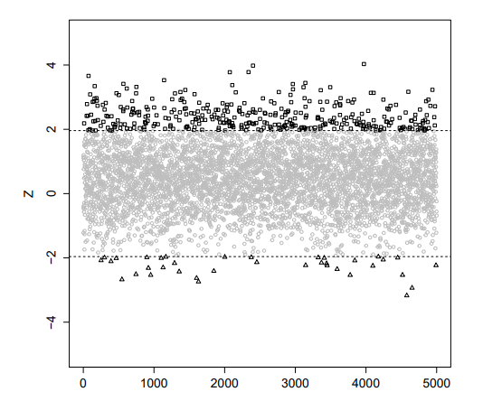
Figure 8.5: (Appeared in Lu, Qiu, and Deng (2018)) Illustration of S and M error from 5000 simulations of a low power (8%) study at the significance level \(0.05\) with small positive true effect. The grey round points correspond to statistically insignificance. The black triangular points correspond to occurrences of the type S error. The black (triangular and squared) points together correspond to occurrences of the type M error (statistically significant but over-estimates the magnitude of the effect)

Figure 8.5 illustrated the two errors. Note that both errors only focus on cases where a rejection decision is made. It can be shown that both errors are a function of power for the two-sided test of ATE. Table 8.4 shows the mapping for moderate powers more than 50% to high powers of 95% in a two-sided test with \(\alpha=5\%\). Type S Error is only an issue when power is very small and practically 0% for moderate power. In fact to illustrate S error in Figure 8.5, the simulation was done with a very low power of only 8%. However, M error is still large for power between 50% to 70%. At 50% power, the exaggeration ratio (M error on average) is 40%! This means at this error, when we observe an estimated ATE \(\Delta\) that rejects the null hypothesis, this \(\Delta\) is on average 40% more than the true ATE \(\delta\). It has a positive bias due to the hypothesis testing selection! Even with a 80% power, the exaggeration ratio is still more than 10%. We found more than 95% power gives 3% exaggeration ratio. If we chose to use a lower p-value threshold \(\alpha=0.005\), as suggested by Benjamin et al. (2018). Table 8.5 shows the exaggeration ratio decreased from 40% to 28% at power 50%, but a power of more than 80% is still needed to keep exaggeration ratio below 10%. This result indicates that if the estimated ATE \(\Delta\) is also important for decision making, the statistical power of 80% is required not just to have a fair chance of detect the effect but also to avoid large over-estimation of the true effect due to the selection bias of picking statistically significant results.

Table 8.4: Mapping from power to exaggeration ratio (expected M Error) and S Error Rate when \(\alpha=0.05\).

Power	Exaggeration Ratio	S Error Rate
50%	40%	<0.01%
60%	29%	\(\approx\) 0%
70%	20%	\(\approx\) 0%
80%	13%	\(\approx\) 0%
85%	9%	\(\approx\) 0%
90%	6%	\(\approx\) 0%
95%	3%	\(\approx\) 0%

Table 8.5: Mapping from power to exaggeration ratio (expected M Error) and S Error Rate when \(\alpha=0.005\).

Power	Exaggeration Ratio	S Error Rate
50%	28%	\(\approx\) 0%
60%	21%	\(\approx\) 0%
70%	15%	\(\approx\) 0%
80%	9.5%	\(\approx\) 0%
85%	7%	\(\approx\) 0%
90%	5%	\(\approx\) 0%
95%	2.4%	\(\approx\) 0%

8.8 Statistical Challenges

In this last section of the chapter, we briefly discuss a few challenges arise in statistical analyses and results interpretation of A/B tests. Challenges listed here are by no means an exhaustive list and many of these challenges also exist in other areas of statistical analysis and not exclusive to A/B tests. Nevertheless, A/B testing really manifested these issues due to its scale, agility, rich data and fluid analysis. Here, we introduce the challenges and mention some existing researches without going into details. More details will be given for some of the challenges in the following chapters.

Multiple Testing. The first challenge is the problem of multiple comparison, or multiple testing. The significance level \(\alpha\) in a null hypothesis testing procedure means if the null hypothesis is true, each test has \(\alpha\) of false rejection. When many tests are done simultaneously, we expect on average a proportion of \(\alpha\) of true null hypotheses being falsely rejected.

Multiplicity in A/B tests takes multiple dimensions. The first is the number of metrics. Each metric represents a different statistical quantity of interest to compare. It is common to have more than 100 metrics and even thousands of metrics. The second dimension is segmentation. The analysis of one metric can be further divide into different tests for different subgroups of the population. The third dimension is number of variant group comparisons. One A/B test can involve more than one pair of comparison when there are multiple treatments (sometimes called an A/B/n test). This is particularly common for early stage experiments, where experimenters want to assess a large number of ideas and filter the candidates down to only a few promising ones. Another dimension is time. Because of the continuous arrivals of new data, the analysis can also be done sequentially. Multiplicity due to time is also known as the issue of Continuous monitoring and Sequential Testing.

There are many known multiple testing adjustment methods, the most well-known and straightforward being the Bonferroni correction, which is to multiply the p-value by the number of multiplicity. These methods are often over-conservative and significantly reduce the sensitivity of a test due to the extremely large number of multiplicity in A/B tests. Methods like false discovery rate (Benjamini and Hochberg 1995) control are less conservative, but the adjustment procedure depends on results of all the tests. In particular, the adjusted results might change if an experimenter decides to add some new segments to analyze.

For continuous monitoring of A/B tests, peaking the results and stop experiment opportunistically is one of the common malpractices. Correct inference has to take each interim analysis into account and in statistics literature this line of researches is called sequential analysis (Bartroff, Lai, and Shih 2012). Johari et al. (2017) applied SPRT (sequential probability ratio test) to the scenario of continuous monitoring in A/B testing and also combined this with multiplicities from other dimensions like the number of metrics being tested simultaneously. Alex Deng, Lu, and Chen (2016) studied this problem from a Bayesian angle.

Selection Bias and Winner’s curse. Multiple testing can be considered as a special case of a broader issue of selective inference. That is, we cast a wide net of a large number of questions to ask, and only choose to pay attention on a small subset of them that are the “most interesting” selected by certain criteria. Typical selection procedures used in A/B tests include looking at results with low p-values, looking through results using different segments or optionally add new segments to create new analyses, checking a group of metrics only when another metric shows “interesting” results, etc. Inference using the same data that the selection was made is problematic similar to the notion of data snooping is bad in machine learning.

Like the training error generally underestimated the true error, post-selection estimates are usually biased. From all metric results from a A/B test, if we select only those with small p-values, the ATE estimator \(\Delta\) are no longer unbiased as it would be without the selection. We introduced Type M error as one way to quantify this bias and we have seen this selection-bias can be quite significant unless the experiment is sufficiently powered to 80% or more. Because of the selection-bias, if we rerun the same experiment again and look at the same \(\Delta\), it is more likely to be smaller in magnitude than the previous run. This phenomenon is also known as “the winner’s curse.”

Correct the selection-bias and more generally provide new statistical inference techniques that take selection and data snooping into account is getting a lot of attention in the statistics community because the trend of big data and cheap computation making post-selection inference a salient issue instead of a “silent scandal.” Researches reinvestigated the Bayesian framework [Senn (2008);Lu and Deng (2016);Efron (2011);] and proposed new frequentist inference techniques like bias estimation and correction [reid2017post;@lee2018winner], data splitting and data carving (Wager and Athey 2017; Fithian, Sun, and Taylor 2014; Taylor and Tibshirani 2015), and applications to high-dimensional statistical model selection (Taylor and Tibshirani 2018; Taylor and Tibshirani 2015; R. F. Barber and Candes 2016) all came out in recent years.

Heterogeneous Treatment Effect. Although the average treatment effect for a metric is often the first thing experimenters care about and so far we have been focusing on ATE estimator \(\Delta\) in this chapter, it is common sense that individual treatment effect varies: Different subjects reacts to the same change in a different way. Individual treatment effects can vary in magnitude, and also in direction. It is very valuable for experiments to be able to understand how treatment effect varies across several dimensions of the subjects, and be able to find insights explaining why different sub-populations respond to the same change in opposite directions.

Time is another important dimension. Many changes have different effect in week days and weekends, and also during work hours and after-work hours. Some treatment might also display novelty effect. A common novelty effect is when a big change is introduced and users need some time to learn the change, in that case initially there might be increased usage such as visits and clicks but the effect decays after users get used to the change. Novelty effect is important because it is not unusual for a change to initially attracts more usage but eventually reduce to mediocre or even negative effect.

There are several challenges in detecting and explaining Heterogeneous treatment effect (HTE):

1. High dimension with low signal noise ratio. There are many ways to split the total population into different sub-populations. Because A/B testing typically have low signal noise ratio and we even struggle to improve sensitivity to detect the average treatment effect for the whole population, analyze a large number of sub-populations both decrease the signal noise ratio (since sample sizes are smaller for sub-populations) and increase multiplicity in the multiple testing challenge.
2. Interoperability and actionability. In an experiment with a lot of metrics, experimenters are dealing with large streams of information from each A/B test. Introducing HTE will further introduce more insights for experimenters to consume. It is crucial for these insights to be actionable, that is the experimenters can interpret the results and know how to take action based on the insight. This means the HTE results need to be high fidelity and low chance of being a noise, and the HTE structure is memorable and make sense.

Long-Term Effect and Feedback Loop. Novelty effect is a time-dependent heterogeneous treatment effect that can be studied in a short period experiment such as weeks. Long-term effect considers the effect of a change after a longer period of months. It is expected that some types of behavior can only be changed through a long time of exposure to a change. Hohnhold, O’Brien, and Tang (2015) gave an example that improving ads quality by removing lower quality ads in search engine results can reduce users’ “ads blindness” and encourage them to click ads more. The effect of removing low quality ads have a negative effect on the revenue in the short-term, but pays off in the long-term when user clicks high quality ads more. Gomez-Uribe and Hunt (2016) also mentioned that certain changes may have a long feedback loop where a change also impacts other components in the system that can eventually impact the effect of the initial change itself. Take online ads as an example, changing ads quality threshold also will change click-through-rate prediction algorithm, which can also impact the ads defect rate estimation algorithm. Feedback loop can also be external. Because one is often not the only player in the market, an introduced change can cause a shock in the market and takes time to reach to a new equilibrium. Understanding long-term effect is difficult. Running a long experiment of months is against agility, and takes bigger effort to make sure the experiment won’t be polluted by various data quality issues, human errors like interaction and conflict with other experiments, as well as technical issue such as cookie churn being a much bigger problem.

Violation of SUTVA Assumption, Leakage and Network Effect. The stable unit treatment value assumption (SUTVA) is an important assumption in the potential outcome framework. It is the reason why we usually can talk about a counterfactual pair instead of a counterfactual vector. Under SUTVA, the potential outcomes of one unit cannot be affected by the assignment of other units, and hence a unit’s potential outcomes only has the degree of freedom equal to that of the treatment assignments. When there is only one treatment, the potential outcomes for any unit is only a pair. Without SUTVA, the potential outcomes for each unit depends on the whole treatment assignment configuration of all units! For a study of n units, one treatment and control creates \(2^n\) different assignment configurations, and we need to consider a potential outcome vector of dimension \(2^n\)! What a life saver the SUTVA is!

However, there are known cases when SUTVA is considered too restrictive and not appropriate. The most notable example is network effect. When there is a network structure connecting a population, the treatment effect for a unit may depend on behaviors of units in the neighborhood, and their behaviors are affected by their treatment assignments! The ideal treatment effect we want to infer is to compare the counterfactual where all units are assigned treatment to the other extreme when all units are in control.

Another issue is leakage effect, where SUTVA is violated in the way that units assigned to control will be affected by treatment units. For example, in skill matching of an online shooting game, any change in the matching algorithm will affect all gamers matched together. If the treatment algorithm tweak a stronger gamer into a lower skill level, they will get an easier game but other gamers at that level will be facing harder opponents. Another example is when the treatment and control are running in a combined environment with shared hardware resources, a treatment using more hardware resources can negatively affect control by starving its resources. In this case both treatment and control will be slowed down.

External Validity. All A/B testing relies on a leap of faith in External validity. That is, we believe the results we learned in one experiment will carry over into the future for the same population we experimented at a different time. Nevertheless, there are cases we intentionally run experiment on one population and want to project the result to a different population. For one example, beta users are willing to participate in active software or firmware update which make them a good population to test client side software such as operation system. But beta users are very different from the general public users. They probably are more technically savvy, have better hardware and network, or the devices joined the beta program are simply not mission critical. In these cases, external validity remains a big issue and we need to adjust the estimation to account for the differences in populations.

---

17. http://en.wikipedia.org/wiki/German_tank_problem↩︎

18. Due to the limitation of user tracking, when cookie is used for user tracking, some level of experience fragmentation is still expected. But at least that experience discontinuity only happens when users change browsers or devices.↩︎

19. Y \(\sim\) Treatment + (1|User) in lme4 notation. A detailed discussion is beyond the scope of this paper; see Gelman and Hill (2006),Bates et al. (2014).↩︎

20. We do not consider cases when \(Y\) has discrete mass, and \(F\) will have jumps. In this case the percentile can take many values and is not well defined. In practice this case can be seen as continuous case with simple discrete correction.↩︎

21. When p is 0.5, the 50% quantile, or median, is often defined as the average of the middle two numbers if we have even number of observations.↩︎

22. The rigorous proof involves a rather technical next step that is beyond our scope. A formal proof can be found in Van der Vaart (2000).↩︎

23. Alex Deng, Knoblich, and Lu (2018) called it outer-CI as the independent case is related to the outer-CI method (Krewski 1976; Meyer 1987).↩︎

24. Both Frequentist and Bayesian.↩︎