Chapter 4 Potential Outcomes Framework
Consider a binary \(Z= 0, 1\) for control and treatment and we are interested in knowing the effect of \(Z\) on an outcome variable \(Y\). The potential outcome framework, also called Rubin-Causal-Model (RCM), augments the joint distribution of \((Z,Y)\) by two random variables \((Y(1),Y(0))\) — the potential outcome pair of \(Y\) when \(Z\) is \(1\) and \(0\) respectively.7 Since \(Y\) is the observed outcome and by definition we have \[\begin{equation} Y = \left \{ \begin{array}{ll} Y(1) & \quad \text{if } Z = 1, \\ Y(0) & \quad \text{if } Z = 0 \end{array} \tag{4.1} \right. \end{equation}\] When \(Z=1\), \(Y(0)\) is not observed and is the counterfactual, and when \(Z=0\), \(Y(1)\) is the counterfactual. Some authors prefer to use \(Y^{\textrm{obs}}\) in place of plain \(Y\) to emphasize it is the observable and the above equation can be made more compact as \[\begin{equation*} Y^{\textrm{obs}} = Z\cdot Y(1) + (1-Z)\cdot Y(0). \end{equation*}\]
At the first look the introduction of counterfactual seems useless because it represents something that we don’t and can’t observe. They will not help us directly to estimate causal effect because we won’t be able to use any formula made of \(((Y(1),Y(0))\) if we don’t have observations to plug into the formula. Nevertheless, the introduction of potential outcome allows statisticians to conduct rigorous causal inference under the familiar joint probability distribution. Under the potential outcomes framework, the problem of identifying a causal effect becomes the challenge of inferring quantities about unobserved counterfactual using only observed.
As the first step, now we can define causal effect rigorously. In the binary \(Z\) case, we call state \(1\) treatment and \(0\) control, and let \[\begin{equation} \tau = Y(1) - Y(0), \tag{4.2} \end{equation}\] to be the treatment effect of changing \(X\) from control to treatment, or simply the treatment effect of \(Z\).
It should be noticed that potential outcome pair is a pair of random variables and treatment effect \(\tau\) is also random. Usually \(Y\) represents certain measurement for an individual subject or unit, such as a person. When we randomly sample a unit from a population, the observation, denoted by \(Y\), is random. The treatment effect \(\tau\) of \(Z\) on \(Y\) is also random. We define the (population) average treatment effect (ATE) to be \[\begin{equation} \mathrm{E^*}(\tau) = \mathrm{E^*}\left(Y(1) - Y(0)\right) \tag{4.3} \end{equation}\]
We emphasize again Equation (4.3) cannot be directly used because we do not observe \(Y(1)\) and \(Y(0)\) simultaneously. We only observe \(Y(1)\) for treatment and \(Y(0)\) for control. In (4.3) we used the superscript \(*\) as a reminder that the expectation is taken under the augmented joint distribution \(P^*\), not the original joint distribution \(P\).
ATE is the most common causal estimand used in practice, as it stands for the expected effect for a random units in a population. When given a sample of \(N\) units \(Y_i, i=1,\dots,N\), we define the sample average treatment effect (SATE) to be \[\begin{equation} \sum_i\left(Y_i(1) - Y_i(0)\right) /N \tag{4.4}. \end{equation}\] SATE is the population average treatment effect (PATE) when the population is fixed to be the given sample. SATE is still a popular causal estimand in literature largely influenced by statistics pioneers like Fisher and Neyman in the complete randomized experiment setting. In this chapter we use ATE almost exclusively for population average treatment effect (PATE) (4.3).
4.1 Naive Estimation
A naive attempt to estimate The ATE \(\mathrm{E^*}(\tau)\) is to use the following \[\begin{equation} \widehat{\tau}_\text{naive} := \overline{Y_T} - \overline{Y_C} \tag{4.5}, \end{equation}\] where \(\overline{Y_T}\) is the average of treatment observations and \(\overline{Y_C}\) for control. We call (4.5) the naive estimation.
\(\overline{Y_T}\) is an unbiased estimate of \(\mathrm{E}(Y|Z = 1)\) and \(\overline{Y_C}\) is an unbiased estimate of \(\mathrm{E}(Y|Z = 0)\). Therefore the naive estimation (4.5) is an unbiased estimator of \[\begin{equation} \mathrm{E}(Y|Z = 1) - \mathrm{E}(Y|Z = 0) \tag{4.6}. \end{equation}\]
(4.6) is called the association effect of \(Z\) on \(Y\). Unlike the causal effect (4.3), association can be defined using the observed joint distribution \(P\).
In general, association (4.6) and causation (4.3) are different, because \(\mathrm{E^*}(Y(z))\) and \(\mathrm{E}(Y|Z = z)\) are not the same. This is just another version of correlation does not imply causation. Associations can be caused by many confounders other than the cause of interest \(Z\). Figure 4.1 demonstrates this using causal graphical models. We will wait until section 5 to introduce causal graphical model. But the idea is very clear in Figure 4.1. There is a potential causal link from \(Z\) to \(Y\). But there might exist confounder \(U\) which can impact \(Z\) and \(Y\) simultaneously.
Figure 4.1: Confounder.
Confounders are the main hurdle of causal inference and why causal inference without randomized experiments are difficult. It is now a common belief that smoking can cause lung cancer. The link between smoking and lung cancer had been suspected for a long time based on many observational studies. But none of them are as definitive as a randomized experiment because it is just impossible to randomize people and force them to smoke or not smoke. Fisher, who popularized randomized experiments in statistics and well understood correlation does not imply causation, publicly spoke out against a 1950 study showing a positive association between smoking tobacco and lung cancer (R. Fisher 1958). One of his arguments, is that there may be a genetic predisposition to smoke and that genetic predisposition is presumably also linked to lung cancer. In other words, there might exist a gene, a confounder that both increase a person’s tendency of smoking and the likelihood of developing lung cancer.
4.2 Randomization and Unconfoundedness
Despite not generally applicable, the naive estimation is the basis of more sophisticated method. Equipped with the potential outcome framework, we not only can clearly see the difference between association and causation, but are also able to further develop methods that can help us isolate confounding effects to recover causal effect. The distinction of \(P\) and \(P^*\), hence \(\mathrm{E^*}\) and \(\mathrm{E}\) is precisely what we need to conquer.
Fortunately, under certain conditions, we can rewrite a causal quantity defined with counterfactuals in the augemented world, e.g. involving \(P^*\) and \(\mathrm{E^*}\), into a form that only involves \(P\)(and/or \(\mathrm{E}\)). The latter can in turn can be estimated with observations since they were drawn from \(P\). In these cases, we say the causal quantity of interest can be identified and we have an identification strategy.
We already know randomization dispels all confounders and naive estimation works in randomized experiments. We first generalize the idea of randomization in the following definition of unconfoundedness, also called ignorability.8First, randomization implies unconfoundedness. Recall independence means \(Z\) is irrelevant for predicting \((Y(1),Y(0))\). For all three randomization mechanisms mentioned earlier, treatment assignment \(Z\) is produced using an exogenous procedure (complete randomization, independent randomization, cluster randomization) totally unrelated to anything else. Knowing the value of \(Z\) lends us no extra knowledge toward predicting \((Y(1),Y(0))\) since the distribution of potential outcomes in different treatment groups are still the same. Unconfoundedness (4.7) is the mathematical incarnation of all-other-thing-being-equal!
Secondly, association implies causation without confounding. To see that, \[\begin{equation*} \mathrm{E}(Y|Z = 1) = \mathrm{E^*}(Y(1)|Z = 1) = \mathrm{E^*}(Y(1)), \end{equation*}\] where the first equality is from the definition (4.1) and the second is from \(Z\) independent of \(Y(1)\). Similarly, \[\begin{equation*} \mathrm{E}(Y|Z = 0) = \mathrm{E^*}(Y(0)). \end{equation*}\] Put them together, \[\begin{equation*} \mathrm{E^*}(\tau) = \mathrm{E^*}\left(Y(1) - Y(0)\right) = \mathrm{E}(Y|Z = 1) - \mathrm{E}(Y|Z = 1). \end{equation*}\] We’ve derived the equivalence between causation (4.3) and association (4.6). Since naive estimation (4.5) unbiasedly estimate association, it also is unbiased for ATE, under the condition of unconfoundedness.
Let us take a second look at the simple proof as it contains the essence of potential outcome framework. The ATE (4.3), defined with counterfactual, can be rewritten as the difference of two conditional expectations involving only observables. This key transition hinges on the additional assumption being made regarding the independence between \(Z\) and \((Y(1),Y(0))\). As we will shortly see, \(Z\) and \((Y(1),Y(0))\) being independent is not the only condition that allows such transition from potential outcome distribution \(P^*\) to observation distribution \(P\).
4.2.1 Conditional Unconfoundedness, Matching and Covariates Balancing
Unconfoundedness seems too restrictive to be applicable to anything beyond randomized experiments. In most observational studies, confounders do exist. Such cases require us to isolate confounding effects. This can be achieved by conditioning on confounders, leading to the concept of conditional unconfoundedness.
Covariate is often very easy to find as they generally represent side (exogenous) or baseline or pre-treatment information. For this reason they are also called attributes or pre-treatment variables. In the kidney stone example, patients’ stone size prior to being treated is a pre-treatment variable, and therefore cannot be affected by the choice of treatments. Discrete covariates are also commonly referred to as segments or strata.
As the name suggests, Definition 4.3 is a conditional version of Definition 4.1. Conditional unconfoundedness means all confounders have already been identified and accounted for by the set of covariates \(X\).9 When covariates \(X\) are all discrete, within any given stratum \(X = x\), there is no confounding effect remains and causal effect can be identified by naive estimation. The overall ATE can be identified by aggregating over all strata. The procedure of forming strata and using naive estimation within each strata is called matching. The following derivation assuming discrete \(Z\) and \(X\) provides a rigorous proof10.
Under the assumption of conditional unconfoundedness, \[\begin{align} P^*(Y(1) = y) & = \sum_x P^*(Y(1)=y |X=x)P^*(X=x) \notag \\ & = \sum_x P^*(Y(1)=y |X=x, Z=1)P^*(X=x) \notag \\ & = \sum_x P^*(Y = y |X=x, Z=1)P^*(X=x) \notag \\ & = \sum_x P(Y = y |X=x, Z=1)P(X=x). \tag{4.9} \end{align}\] The second equality is from (4.8). The last equality is from the fact that \(P\) and \(P^*\) are the same for all observables \(X\), \(Z\) and \(Y\). Similarly \[\begin{equation} P^*(Y(0) = y) = \sum_x P(Y = y |X=x, Z=0)P(X=x). \tag{4.10} \end{equation}\]
For ATE \(\mathrm{E^*}\left(Y(1) - Y(0)\right)\), from (4.9) and (4.10) \[\begin{align} &\mathrm{E^*}\left(Y(1) - Y(0)\right) \notag \\ & = \sum_x \left(\mathrm{E}(Y = y |X=x, Z=1) - \mathrm{E}(Y = y |X=x, Z=0)\right)\times P(X=x). \tag{4.11} \end{align}\]
Let \(\overline{Y_T(x)}\) and \(\overline{Y_C(x)}\) be the sample average of observed \(Y\) in treatment and control groups for a stratum \(X = x\) and \(\widehat{\mu}_\text{naive}(x) = \overline{Y_T(x)} - \overline{Y_C(x)}\) be the naive estimation on the stratum. Also let \(\widehat{p}(x)\) be the proportion of stratum \(X = x\) in the total observations. An unbiased estimate for ATE in the form of (4.11) is \[\begin{equation} \widehat{\mu}_\text{match} : = \sum_x \widehat{\mu}_\text{naive}(x) \times \widehat{p}(x). \tag{4.12} \end{equation}\]
We call Equation (4.12) the (exact) matching estimate. It is a sum of naive estimations weighted by the observed proportion of each stratum \(X=x\). Intuitively we are matching subjects having the same covariates \(X\).
In the kidney stone example, we already identified pre-treatment stone size as a possible confounder. Matching on kidney stone means comparing two treatment on each stone size group separately and then aggregate up to get an overall estimate for all patients. This will resolve the Simpson’s paradox as shown in Table 2.1.
The obvious challenges regarding matching estimator (4.12) is that naive estimation for each stratum requires a reasonable number of units in each stratum. In other words, how many units can we match together for each different values of \(X\). If the matching produce sparse strata, i.e. those with small number of units either from treat or control group. The naive estimation for these strata would have high variance, making the overall ATE estimation high variance too. This kind of sparseness can easily happen if one covariate have too many levels or be continuous, or if we put too many discrete covariates in \(X\) so the total number of combinations is large.
To overcome sparseness after matching, one approach is to notice that it is not necessary to match perfectly on every individual levels of \(X\). The rationale behind matching is that when confounders exist, we want to isolate confounding effects so that any correlation (association) between \(Z\) and \(Y\) cannot be attributed by correlation of \(Z\) and any confounder. Fixing the value of confounder by exact conditioning certainly can make sure \(Z\) is independent of all confounders (any random variable is independent of a fixed value). But this is sufficient but not necessary. All we need to make sure is \(Z\) is independent of confounders \(X\). When \(Z\) is independent of \(X\), the distribution \(X\) and conditional distribution of \(X\) given \(Z\) are the same. Equivalently speaking, the distribution of \(X\) for control group \(Z=0\) and the distribution for treatment group \(Z=1\) are the same. In this sense there should be no difference in the distribution of any confounders in \(X\) between the two groups and the two groups should be balanced for covariates \(X\). This suggests it is sufficient to form strata such that distribution of covariates \(X\) is balanced between treatment and control and conditioning on the strata.
Being a function of \(X\), \(b(X)\) will be coarser than \(X\). When \(X\) are all discrete, \(b(X)\) is also discrete and will have less number of levels than \(X\). Theorem 4.1 says \(b(X)\) is all we need to condition on for naive estimation to work. For the purpose of matching, we only need to match on a balancing score \(b(X)\).
Note \(b(X)\) might not be univariate. (e.g. The trivial case \(b(X) = X\) when \(X\) is multivariate.) When \(X\) are discrete, we derive a special balancing score called propensity score. In the next section we show how to extend propensity score to general continuous case and prove the optimal property of propensity score as the coarsest balancing score.
Let \(N_T(x), N_C(x), N(x)\) be the sample sizes of treatment, control, and total size for the stratum \(X = x\). Let \(N\) be the total sample size. Then \(\widehat{p}(x) = N(x)/N\).
Define the propensity score \(e(x)\) to be \(N_T(x)/N(x)\). \(e(x)\) is the proportion of samples within the stratum \(X = x\) that are in the treatment group. Let \(N(e)\), \(N_T(e)\) and \(N_C(e)\) be sample sizes when stratified by the propensity score, i.e. \[\begin{equation*} N_T(e) = \sum_{e(x) = e} N_T(x),\quad N_C(e) = \sum_{e(x) = e} N_C(x), \\ N(e) = \sum_{e(x) = e} N(x). \end{equation*}\] We can reorganize the matching estimator as the following. Let \((X_i, Z_i, Y_i), i=1,\dots,N\) be the observations. \[\begin{align} \sum_x & \widehat{\mu}_\text{naive}(x) \times \frac{N(x)}{N} = \frac{1}{N} \sum_x \left (\frac{\sum_{X_i = x, Z_i = 1} Y_i}{N_T(x)/N(x)} - \frac{\sum_{X_i = x, Z_i = 0} Y_i}{N_C(x)/N(x)}\right) \notag \\ & = \frac{1}{N}\left ( \sum_{Z_i = 1} \frac{Y_i}{e(X_i)} - \sum_{Z_i = 0} \frac{Y_i}{1-e(X_i)} \right). \tag{4.14} \end{align}\] We now regroup samples by their values of \(e(X_i)\), and noting \(N_T(e)/N(e) = e\), \(N_C(e)/N(e) = 1-e\), (4.14) equals \[\begin{align} & \frac{1}{N}\sum_e\left ( \sum_{e(X_i) = e, Z_i = 1} \frac{Y_i}{e} - \sum_{e(X_i) = e, Z_i = 0} \frac{Y_i}{1-e} \right)\notag\\ & = \frac{1}{N}\sum_e\left ( \sum_{e(X_i) = e, Z_i = 1} \frac{Y_i}{N_T(e)/N(e)} - \sum_{e(X_i) = e, Z_i = 0} \frac{Y_i}{N_C(e)/N(e)} \right)\notag \\ & = \sum_e\left ( \left ( \frac{\sum_{e(X_i) = e, Z_i = 1} Y_i}{N_T(e)} - \frac{\sum_{e(X_i) = e, Z_i = 0} Y_i}{N_C(e)} \right) \times \frac{N(e)}{N} \right) \notag \\ & = \sum_e \left (\widehat{\mu}_\text{naive}(e) \times \frac{N(e)}{N} \right ).\tag{4.15} \end{align}\] (4.15) is the exact matching estimator when matched by \(e(X)\) instead of \(X\) directly. (4.14) has a form of weighted average of \(Y_i\). Make a note of this form as we will return to this very soon.
There is an intuitive connection between propensity score stratification and randomized experiment. We have seen unconfoundedness allows us to treat the observed data as if it were collected from a randomized experiment and use the naive estimation to unbiasedly estimate ATE. Conditional unconfoundedness is weaker for that unconfoundedness holds only for every stratum \(X = x\). Within each stratum, we can pretend the data to be collected from a randomized experiment using independent randomization, with probability \(e(X)\) to be assigned to treatment. In this connection, conditional unconfoundedness allows us to pretend the data set \((Y_i, X_i, Z_i)\) was collected using a conditional randomized experiment, in which for each given \(X\), a unit has a probability \(e(X)\) to be assigned to treatment. It is easy to see that we can reduce the complexity of these conditional randomized experiments by combining strata with the same \(e(X)\) together as one randomized experiment because the assignment probabilities are the same. This reduction is also the optimal in the sense we cannot combine two randomized experiment with two different assignment probabilities together. (4.15) is a direct consequence from the conditional randomized experiment view.
4.3 Propensity Score
Under the conditional unconfoundedness assumption (4.8), define propensity score to be a function of covariates \(X\) as \[\begin{equation} e(X) := P(Z = 1 | X) \tag{4.16}. \end{equation}\] That is, \(e(X)\) is the probability a unit will be associated with \(Z=1\) (be treated) conditioned on the given \(X\). It is also the expected proportion of units with \(Z=1\) among units with the same value of \(X\). The following theorem says propensity score is the best balancing score.
Theorem 4.2 says not only is the propensity score \(e(X)\) a balancing score, it is the coarsest one possible. Also this definition works for both discrete or continuous covariates.
Proof. We only need to prove the second part. The first part follows directly from the second part by realizing \(e(X)\) is \(\mathit{id}(e(X))\) for the identify function \(\mathit{id}\).
For the if part, if \(e(X) = f(b(X))\), we need to show the distribution of \(Z\) given \(X\) and \(e(X)\) is the same as the distribution of \(Z\) given only \(e(X)\). Since \(Z\) is binary, we only need to show \[\begin{equation} P(Z = 1 | X, e(X)) = P(Z=1|e(X)). \tag{4.17} \end{equation}\] For the LHS \(P(Z=1|X, e(X)) = P(Z = 1 | X) = e(X)\) because \(e(X)\) is redundant given \(X\).
For the RHS, \[\begin{align*} P(Z=1|e(X)) = \mathrm{E}\left( \mathbf{1}_{Z=1} | e(X) \right) = \mathrm{E}\left( \mathrm{E}\left( \mathbf{1}_{Z=1} | X, e(X) \right) |e(X) \right) \\ = \mathrm{E}\left( e(X) | e(X)\right) = e(X). \end{align*}\] LHS = RHS, hence \(e(X)\) is a balancing score.
For the only if part. If \(e(X)\) is not a function of \(b(X)\), then there must exists two \(x\) and \(x'\) such that \(b(x) = b(x')\) but \(e(x)\neq e(x')\).
We proved the RHS of (4.17) is \(e(X)\). So RHS is not the same for \(X = x\) and \(X = x'\).
The LHS of (4.17) is \(P(Z = 1 |X)\) and by definition of balancing score, \(P(Z = 1 |X) = P(Z = 1 |b(X))\). Therefore LHS for \(X = x\) and \(X = x'\) must be the same if \(b(x) = b(x')\).
We have reached a contradiction. Hence (4.17) must be false.Propensity score plays a central role in matching and covariate balancing. Under the conditional unconfoundedness assumption, matching on the propensity score is equally good at removing confounding effect as matching on all confounders. It reduces the dimension of matching from arbitrary high dimension to only one dimension. Being the coarsest balancing score, propensity score provides the largest sample size for each matched stratum.
When \(X\) is continuous, \(e(X)\) could still be continuous. Exact matching on even a univariate continuous scale is sparse.
There are two options in general. First option is to forgo exact matching. Approximate matching can be performed using a distance metric such as Mahalanobis distance to match each unit with its nearest neighbors. For a univariate matching score, simple discretization is also used. In both cases the unbiasedness property of the matching estimator will be disturbed and it is a price to pay for more robust estimator. More on bias-variance trade off in Section 4.10.
Fortunately, propensity score can also be used beyond exact matching. We can treat propensity score, or more exactly the inverse of propensity score, as a reweighting of samples. This perspective is closely connected to importance sampling in Monte Carlo simulation, and missing data perspective of the potential outcome framework. See Section 4.8.
In the next section, we have to talk about the single most important assumption underneath the potential outcome framework — the Stable Unit Treatment Value Assumption, or SUTVA.
4.4 SUTVA
Potential outcome framework naturally extends to non-binary treatment \(Z\) and even continuous \(Z\). In this case we define \(Y_z\) as the potential outcome of \(Y\) if \(Z = z\). Equation (4.1) becomes \[ Z = z \Rightarrow Y_z = Y. \] Keen readers may have sensed the potential outcome framework as we presented seems to be oversimplified. Indeed it is not complete unless we bring up the following key assumption called stable unit treatment value assumption.In a nutshell, SUTVA means there is no interference between different observations. Let \(X\) be binary for illustration and there are two observations \((Y_1, Z_1)\) and \((Y_2,Z_2)\). If the potential outcomes of the first observation depends not only on \(Z_1\) but also on \(Z_2\), then there are 4 total scenarios! We would need 4 potential outcomes for \(Y_1\), and similarly for \(Y_2\). Often the total number of observations can be much larger, leading to a huge number of treatment assignment scenarios — all combinations of the assignment vector \(\mathbf{Z}\). Without SUTVA, the dimensionality of potential outcomes for each unit can be easily unmanageable even for a handful of observations. Moreover, it also increases when number of units increase. Both the model and math required to analyze it easily gets complicated and unwieldy. For this reason, SUTVA is the implicit assumption underneath most results developed under the potential outcome framework. When there is no mention of SUTVA, we should still treat SUTVA as an assumption when using potential outcome framework, unless interference or violation of SUTVA is explicitly called out.
SUTVA should not be confused with independent observations assumption. For a simple example, consider a binary treatment with constant treatment effect. e.g. \(Y(1) = Y(0) + \mu\). SUTVA is satisfied here even when \(Y(0)\) of different units can be dependent and therefore observation \(Y_i\)s are not independent of each other.
In practice, independence is still a common and reasonable assumption to make, or at least we assume independence at some level that might be different from the original analysis unit. For example in cluster randomized experiment, clusters are typically assumed to be independent of each other, even though the clustering might introduce dependencies between analysis units.
4.5 Missing Data and Weighted Samples
In the previous sections we’ve seen how the potential outcome framework work leads us to the matching estimator (4.12). We relies a bit on rigorous mathematical derivations and didn’t spend much time explaining the natural intuition. Here is a recap of what we did
- We introduced potential outcomes by augmented the joint distribution of observed by unobserved counterfactuals.
- We defined causal effect such as ATE under the augmented joint distribution \(P^*\).
- We identified conditional unconfoundedness as the condition under which we can express ATE using only the joint distribution \(P\) for the observed, leading to matching estimator.
- We show exact matching can be relaxed to matching on a balancing score. Propensity score is the coarsest balancing score.
Starting from this section we take another look at potential outcomes using a slightly different, more intuitive yet mathematically equivalent view. Instead of focusing on the distinction between the augmented joint distribution \(P^*\) and original distribution \(P\), we just treat \(P^*\) as the only joint distribution governs all observations. However, we treat the unobserved counterfactuals as missing data! To be specific, we assume there is an oracle that observed all potential outcomes. But after she observed everything, she will remove all counterfactuals and keep only the potential outcome associated with the observed assignment.
What’s the difference between the two views? Mathematically they are equivalent, just two different ways of telling the story of the same data-generating-process. In the augmented joint distribution view, we need to keep two distributions in check. We use \(P^*\) to define causal estimands, and \(P\) to form estimates. And we need to consciously keep track of whether we can re-express any estimands defined in \(P^*\) using \(P\). In the missing data perspective, there is only one distribution — \(P^*\) to keep in mind. The difficulty lies in the fact some observations are missing and we need to do inference about \(P^*\) using observed data only.
In the authors’ subjective opinion, there are a few advantages of the missing data perspective:
- The idea of missing data is easier to apprehend and convey without using heavy math notations. Concepts like missing completely at random speaks for itself.
- Missing data is an important problem occurring in many fields. There are many theories and results existed.
- Missing data naturally connects the concepts of randomness (missing at random), sample reweighting, and missing data imputation together.
4.6 Missing Data Mechanisms and Ignorability
Let \(Z\) be the indicator of missingness for an observation \(Y\). \(Z=1\) if \(Y\) is observed and \(Z=0\) if missing.
In particular, \(Y \perp \! \! \! \! \perp Z\).
There is a clear connection between MCAR and unconfoundedness (4.7), and MAR and conditional unconfoundedness (4.8). The difference is there is no potential outcome pair \((Y(1),Y(0))\), just one \(Y\). More specifically, when counterfactuals are MAR, both \(Y(1)\) and \(Y(0)\) are MAR. Therefore, \[ Y(1) \perp \! \! \! \! \perp Z | X, \quad \text{and} \quad Y(0) \perp \! \! \! \! \perp Z | X, \] which is weaker than the conditional unconfoundedness condition \[ (Y(1),Y(0)) \perp \! \! \! \! \perp Z | X, \] but is equally powerful for majority of cases.
Exercise: Show \(A \perp \! \! \! \! \perp X\) and \(B \perp \! \! \! \! \perp X\) does not imply \(A,B \perp \! \! \! \! \perp X\).
The name ignorability for unconfoundedness and strong ignorability for conditional unconfoundedness are better understood using missing data perspective. In both cases it refers to the notion that the fact there are missing data can be ignored as if they are complete data. This is obvious if missing data is MCAR because the observed data distribution is the same as the complete data distribution. For MAR, the missing data is ignorable within each stratum. But the probability of missing may vary from stratum to stratum. This means for MAR, within each stratum, the distribution of observed data represents the distribution of the complete data. But when all strata combined together, the proportion or weight of each stratum for observed data is different from that of the complete data, because some strata have more data missing while some have less. In other words the weights of different strata are skewed due to different impact of data missing. If we can correct the observed weights into their original weights in the complete data, then we will be able to correct the distribution of observed data so that it faithfully represents the complete data distribution. How should each stratum be reweighted? If the missing rate for a stratum is higher than average, then it is more impacted by the missing event, and hence under-represented in the observed data. If missing rate is lower than average, this stratum will be over-represented. This is the key observation leads to the inverse propensity score weighting (IPW).
The idea of reweighting comes from importance sampling in Monte Carlo simulation. It is an essential concept and a must-have tool in every data scientist’s toolbox. We will talk about it first before returning to inverse propensity score weighting in Section 4.8.
Here is a short summary of connections among randomized experiments, unconfoundedness and missing data we have observed so far:
- Randomized Experiment \(\implies\) unconfoundedness/ignorability \(\iff\) \(Y(1)\) and \(Y(0)\) are MCAR
- Conditional Randomized Experiment \(\implies\) conditional unconfoundedness/strong ignorability \(\iff\) \(Y(1)\) and \(Y(0)\) are MAR
- If \(Y(1)\) is MAR, the event of \(Y(1)\) missing follows an independent Bernoulli distribution with the probability equal to the propensity score \(e(X) = P(Z = 1 |X)\). Similarly, \(Y(0)\) follows the same distribution with probability \(1-e(X)\) of missing.
- Under MCAR the fact that there are data missing can be ignored. For MAR, the impact of missing data is measured by the propensity score.
4.7 Importance Sampling
The idea is that the empirical distribution \(P_n\) provide an unbiased representation of \(P\) and it converges to \(P\) as \(n\) increases. A rigorous understanding of the convergence here requires theories like Glivenko–Cantelli theorem and Donsker’s theorem; see endnotes. Heuristically speaking, the histogram of \(X_i, i=1,\dots,n\) must converge to the density function of \(P\). This heuristics suggest that for estimating any quantity defined by the theoretical distribution \(P\), a natural estimator is to replace \(P\) with its empirical version \(P_n\). This estimator should be consistent, i.e., it converges to the statistical quantity of interest and asymptotically unbiased if \(P_n\) correctly represents \(P\). It is even better if the estimator after proper standardization could also be asymptotically normal. A set of very useful results from theoretical asymptotic statistics showed our naive wishes are mostly true under mild regularity conditions.
For causal inference, effect on mean and quantiles are of major interest. With i.i.d. sample from \(P\), estimating mean is straightforward.Theorem 4.3 is a direct application of strong law of large numbers. It is the foundation of Monte Carlo Simulation/Integration. For any statistical quantify of interest that can be expressed as an expectation of a, the empirical expectation, i.e. the average \(\overline{f(X)}\), can be used as an unbiased estimator. We can also employ the central limit theorem to see \(\overline{f(X)}\) will be asymptotically normal provided \(f(X)\) has finite variance.
Let \(F\) be the distribution function of \(P\) and \(F_n\) be the empirical version. p-quantile is defined as \(F^{-1}(p)\) and sample p-quantile can be defined as \(F_n^{-1}(p)\).
Theorem 4.4 says for continuous random variable with density function \(f\), the empirical quantile estimator is asymptotically unbiased with normality. For discrete random variable, the empirical quantile estimator is still asymptotically unbiased, but not asymptotically normal because empirical quantile is always discrete. However it should still be close to a normal distribution and we can use continuity correction to make it even closer.
A unified view of both mean and quantile is to treat both as solutions of their own corresponding optimization problems.
Theorem 4.5 Median of a random variable \(X\) with distribution \(P\) is the solution of the following optimization problem: \[ \min_{\theta} \mathrm{E_P}\left( |X - \theta| \right). \]
More generally, the \(p\)-quantile is the solution of \[ \min_{\theta} \mathrm{E_P}\left( \psi(X)\right), \] where \[\begin{equation*} \psi(x) = \left \{ \begin{array}{ll} (1-p)|x| & \quad \text{if } x < 0, \\ 0 & \quad \text{if } x = 0,\\ p|x| & \quad \text{if } x > 0 \end{array} \right. \end{equation*}\]
As a comparison, mean of a random variable \(X\) with distribution \(P\) is the solution of the following optimization problem: \[ \min_{\theta} \mathrm{E_P}\left( (X - \theta)^2 \right). \]Proof of Theorem 4.5 is left as an exercise. Note that the derivative of \(\psi(x)\) is \(-(1-p)\) if \(x<0\), \(p\) if \(x>0\) and the subderivative for \(x=0\) is \([-(1-p), p]\).
Quantile and mean share the same empirical form as the solution of minimizing the expectation of a parameterized function \(\psi_\theta(x)\) of a random variable. By simply replacing the theoretical distribution \(P\) by its empirical version \(P_n\), solving the empirical version of the same minimization problems leads to the empirical mean and empirical quantile.
By the heuristics of \(P_n\) converging to \(P\), we expect the solutions of the empirical problem also converge to solutions of the theoretical problem. This is the topic of M-estimator (and closely related Z-estimator). M-estimators are asymptotically normal under mild assumptions. See Section 11.3.
We saw empirical distribution can be a really powerful aid. But to get an empirical distribution, so far we have been assuming we know how to draw \(i.i.d.\) samples from \(P\).11 In some cases drawing from a distribution \(P\) might be very hard or even infeasible. In a nutshell, importance sampling allows us to represent a distribution empirically using samples drawn from another.
Theorem 4.6 (Change of Measure/Radon–Nikodym) If probability measure \(P\) is absolutely continuous with respect to another probability measure \(Q\), then there exists a random variable \(LR\) such that \[\begin{equation} \mathrm{E_P} \left(f(X)\right) = \mathrm{E_Q} \left( f(X) \times LR \right).\tag{4.19} \end{equation}\] The random variable \(LR\) is called the Radon-Nikodym derivative in measure theory. It is unique up to a null set of \(Q\) (almost surely unique w.r.t. to \(Q\)).
The following special non-measure-theoretic form is sufficient for practice.
If both \(P\) and \(Q\) have density function denoted by \(dP = p(x)\) and \(dQ = q(x)\), and \(q(x) = 0\) always implies \(p(x) = 0\), then \[ LR = \frac{dP(X)}{dQ(X)} = \frac{p(X)}{q(X)} \quad a.s. \] i.e., the Radon-Nykodym derivative is the likelihood ratio.Theorem 4.6 is called change of measure because is transform an expectation under \(P\) using an expectation under \(Q\) by reweighting random variable \(X\) from \(Q\) by the likelihood ratio. The idea is obvious but a rigorous proof requires measure theory and is beyond our scope nor is it essential for data scientists. See the endnotes of this chapter for further readings. Change of measure leads to importance sampling.
Corollary 4.1 (Importance Sampling) If \(X_i, i = 1, \dots, N\), is drawn \(i.i.d.\) from distribution \(Q\) and \[ LR_i = L(X_i) = \frac{dP(X_i)}{dQ(X_i)} \] be the likelihood ratio of \(P\) to \(Q\). Then \[\begin{equation} \widehat{\mu}_\text{IS}:= \overline{f(X)\times LR} = \frac{\sum_i f(X_i) \times LR_i}{N} \tag{4.20} \end{equation}\] is an unbiased estimator for \(\mathrm{E_P}\left(f(X)\right)\).
If only given the likelihood ratio up to a constant, i.e. \[ w_i \propto LR_i = \frac{dP(X_i)}{dQ(X_i)}. \] An asymptotically unbiased self-normalized estimator for \(\mathrm{E_P}\left(f(X)\right)\) is \[\begin{equation} \widehat{\mu}_\text{IS-SN} := \frac{\sum_i f(X_i) \times w_i}{\sum_i w_i} \tag{4.21} \end{equation}\]The self-normalized estimator \(\widehat{\mu}_\text{IS-SN}\) (4.21) is a ratio estimator and is not finite sample unbiased. Nevertheless, it is asymptotically unbiased and converges to \(\mathrm{E}_P\left(f(X)\right)\) almost surely. Both (4.20) and (4.21) are asymptotically normal with additional mild (finite seond moment) conditions.
Given i.i.d. weighted samples drawn from \(Q\), the variance for the importance sampling estimator \(\widehat{\mu}_\text{IS}\) (4.20) is \[\begin{equation*} \frac{1}{N}\left(\mathrm{E_Q}\left( f(X)^2LR^2\right) - \mu^2\right), \end{equation*}\] where \(\mu = \mathrm{E}_P\left(f(X)\right)\). It can be estimated by \(\widehat{\sigma}^2/N\), where \[\begin{equation} \widehat{\sigma}^2 = \frac{1}{N}\sum_{i=1}^N f(X_i)^2LR_i^2 - \overline{f(X)\times LR}^2. \tag{4.22} \end{equation}\] The variance of the self-normalized estimator \(\widehat{\mu}_\text{IS-SN}\) (4.21) is trickier. Using the delta method, the asymptotic variance of \(\sqrt{N}(\widehat{\mu}_\text{IS-SN} - \mu)\) is \[ \mathrm{E_Q} \frac{ \left( (f(X)W - \mu W)^2 \right) }{\mathrm{E_Q}(W)^2} \] and can be estimated by \[\begin{equation} \widehat{\sigma}^2_\text{SN} = \frac{\frac{1}{N} \sum_i w_i^2(f(X_i)-\widehat{\mu}_\text{IS-SN})^2 }{\left(\frac{1}{N}\sum_i w_i\right)^2}. \tag{4.23} \end{equation}\] An approximate variance for \(\widehat{\mu}_\text{IS-SN}\) (4.21) is just \(\widehat{\sigma}^2_\text{SN}/N\).
When using importance sampling (IS), each \(i.i.d.\) observation comes together with a weight \(W_i\) equals the likelihood ratio of the target distribution \(P\) to the operating distribution \(Q\). We call them weighted samples. When weights are integers, this is conceptually equivalent to replicating each observation \(X_i\) for \(W_i\) copies. Note that this conceptual equivalence is only for unbiased representation of the target distribution \(Q\), not including independence since replicas are not independent. The non-integer weights can also be interpreted as replicates as long as you are comfortable with the idea of non-integer number of replicates.
Exercise: how to define sample quantile using weighted samples?
We use Figure 4.2 to illustrate the effect of likelihood ratio reweighting. We first simulate 10,000 i.i.d. samples from Poisson(5) distribution. Top left in Figure 4.2 shows the empirical distribution \(P_n\) in its histogram. If we wish to turn this empirical distribution into a \(Q_n\) that mimics Poisson(3), we need to give each sample \(X_i\) a weight equal to the probability of observing \(X_i\) under Poisson(3) to that under Poisson(5). This is shown in the two lower plots, where probability mass function of Poisson(5) and Poisson(3) are overlaid and the likelihood ratio is shown. The top right is the weighted histogram. We see its shape is very close to the probability mass function of a Poisson(3) distribution, marked by the black points.
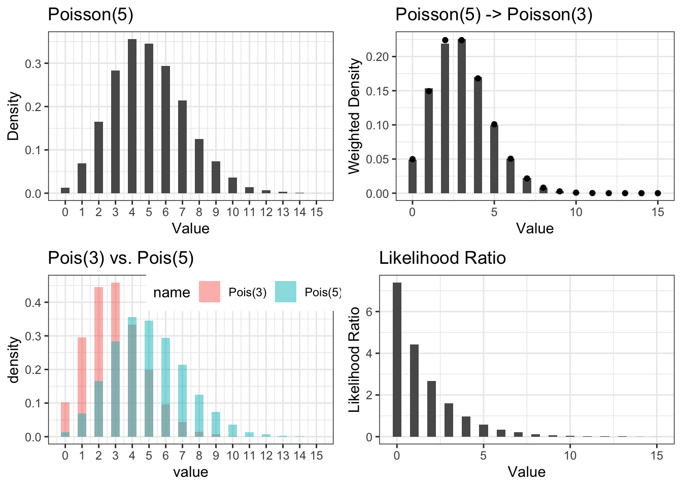
Figure 4.2: Illustration of Importance Sampling to transform a Poisson(5) sample into a weighted sample representing Poisson(3). Top left: Histogram of 10,000 i.i.d. Poisson(5) samples. Top right: Histogram of the 10,000 samples weighted by likelihood ratio of Poisson(3) to Poisson(5) compared to the Poisson(3) density (black points). Lower left: overlay of Poisson(5) and Poisson(3) histograms. Lower right: Likelihood ratio of Poisson(3) to Poisson(5).
Importance sampling and the concept of weighted samples are examples of simple yet powerful ideas. They are widely applied in different theoretical and applied disciplines and essential for every data scientist. We will see how inverse propensity score weighting could be considered as a special case of importance sampling.
4.8 Inverse Propensity Score Weighting (IPW)
Recall the missing data perspective postulate the complete data distribution \(P^*\) where \(Y(1)\) and \(Y(0)\) are all observed no matter \(Z = 1\) or \(Z = 0\). Let \(P\) be the distribution of the observed. Under MAR, we know the observed distribution \(P\) is a skewed version of the complete data distribution \(P^*\) and we also know the mechanism of how it is skewed. IPW is to transform \(P\) back to \(P^*\), so that we can estimate \[ \mathrm{E^*}\left( Y(1) \right)\ \text{and}\ \mathrm{E^*}\left( Y(0) \right). \]
Let’s focus on \(Y(1)\) first as \(Y(0)\) is very similar. From the importance sampling perspective, our observations are samples from \(P\) and our target distribution is \(P^*\). Let \(p\) and \(p^*\) be their densities. The weights should be equal to the likelihood ratio between the two \(\frac{dP^*}{dP} = \frac{p^*}{p}\).
How do we compute the likelihood ratio of \(P^*\) to \(P\)? We need to use MAR. MAR means the data generating process for \(Y\) given \(X\) is independent of the missing process, so we can decompose the density \(p\) as \[ p(x,y) \propto p^*(x,y,z=1) = p^*(x) \times p^*(y|x)\times P^*(z = 1|X=x) = p^*(x,y)\times e(x), \] where \(e(x)\) is the propensity score \(P^*(z=1|x)\). Reorganize this equation leads to \[ \frac{p^*(x,y)}{p(x,y)} \propto \frac{1}{e(x)}. \]
We derived the likelihood ratio to transform \(P\) to \(P^*\) is proportional to the inverse of propensity score! If you are curious to know the normalzation constant, it is \[ \frac{p^*(x,y)}{p(x,y)} = \frac{1}{e(x)} \times P^*(Z = 1) \]
A unbiased estimator for the normalization constant \(P^*(Z=1)\) is simply \(N_T/N\). The importance sampling estimator for \(\mathrm{E^*}\left( Y(1)\right)\) is \[\begin{equation} \widehat{\mu}_{IPW}(Y(1)) = \frac{\sum_{Z=1}Y_i \times \frac{N_T/N}{e(X_i)}}{N_T} = \frac{\sum_{Z=1}{Y_i/e(X_i)}}{N} \tag{4.24} \end{equation}\]
The self-normalized importance sampling estimator is \[\begin{equation} \widehat{\mu}_{IPW-SN}(Y(1)) = \frac{\sum_{Z=1}Y_i/e(X_i)}{\sum_{Z=1} 1/e(X_i)} \tag{4.25} \end{equation}\]
IPW estimator for \(\mathrm{E^*}\left( Y(0)\right)\) is similar with the only notable difference being the likelihood ratio is the inverse of \(1-e(X_i)\), i.e., the propensity of the control observation being missed. The IPW is (4.26) and the self-normalized IPW estimator is (4.27) \[\begin{align} \widehat{\mu}_{IPW}(Y(0)) & = \frac{\sum_{Z=0} Y_i \times \frac{N_C/N}{1-e(X_i)}}{N_C} = \frac{\sum_{Z=0}{Y_i/(1-e(X_i))}}{N} \quad \tag{4.26} \\ \widehat{\mu}_{IPW-SN}(Y(0))& = \frac{\sum_{Z=0} Y_i/(1-e(X_i))}{\sum_{Z=0} 1/(1-e(X_i))} \tag{4.27} \end{align}\]
Unbiased estimator for the ATE can be derived using the difference of unbiased estimator for \(\mathrm{E^*}(Y(1))\) and \(\mathrm{E^*}(Y(0))\). For example, the self-normalized IPW estimator for ATE is \[\begin{equation} \Delta_\text{IPW-SN} = \frac{\sum_{Z=1}Y_i/e(X_i)}{\sum_{Z=1} 1/e(X_i)} - \frac{\sum_{Z=0} Y_i/(1-e(X_i))}{\sum_{Z=0} 1/(1-e(X_i))} \tag{4.28}. \end{equation}\]
The notion of weighted sample and importance sampling can easily allow us to derive causal estimands like average treatment effect of treated (ATT). Let \(P_T\) be the distribution of treated units, i.e. \(P_T(X,Y(1),Y(0)) = P^*(X,Y(1),Y(0)|Z = 1)\). For \(Y(1)\), there is no missing data so IPW is not needed and sample average of treatment observations serves as an unbiased estimate. For \(Y(0)\), the observed distribution is \(P_C(X,Y(0)) = P^*(X, Y(0)|Z = 0)\) and we want to estimate \(\mathrm{E_{P_C}}\left( Y(0)\right) = \mathrm{E^*}\left( Y(0) |Z=1\right)\) using observations from \(P_C\). The likelihood ratio of \(P_T\) to \(P_C\) is \[ \frac{dP_T}{dP_C} \propto \frac{p^*(x)p^*(y|x)p^*(z=1|x)}{p^*(x)p^*(y|x)p^*(z=0|x)} = \frac{p^*(z=1|x)}{p^*(z=0|x)} = \frac{e(x)}{1-e(x)}. \] We can easily transform from \(P_C\) to \(P_T\) by using (unnormalized) importance weight \(\frac{e(x)}{1-e(x)}\). The rest is left as an exercise.
Exercise: Derive normalization constant for \(\frac{e(X)}{1-e(X)}\) w.r.t. the distribution \(P_T\). Derive IPW and self-normalized IPW estimator of \(\mathrm{E_{P_T}}\left( Y(0)\right)\).
4.9 Doubly Robust Estimation
In Section 4.8 we have shown reweighting observed data using the inverse propensity score as weights transforms the observed data into a weighted sample representing the complete data distribution. The purpose of this reweighting/transformation is so that we can infer statistical quantities, e.g. mean and percentiles, of the complete data distribution. In the basic case when the missing data is missing completely at random, the observed data distribution and the complete data distribution are the same — corresponds to a single propensity score for all observed data. In randomized experiments, the designed proportion of each group is the common propensity score.
Reweighting is a powerful tool, but it still relies on missing at random condition, given a set of completely observable covariates \(X\), and a good estimation of the propensity score \(e(X) = P(Z = 1|X)\). An even more naive idea to handle missing data is to impute the missing values, using covariates \(X\) as predictors. For potential outcomes, we want to impute \(Y(1)\) for control units and \(Y(0)\) for treatment units.
Since we do observe \(Y(1)\) and \(X\) for the treatment group, we can surely fit a regression model of \(Y(1)\) on \(X\). For control group, we still observe \(X\). Can we apply the same model we just learned and apply it to the control group to impute missing \(Y(1)\)? The answer is yes under MAR.
Recall under MAR condition, \(Y(1)\) is independent of \(Z\) given \(X\). So knowing \(Z\) will not help us better predicting \(Y(1)\) using \(X\). This suggests that there is no point of applying different regression models of \(Y(1)\) on \(X\) for the cases of \(Z=1\) and \(Z=0\)!
By the same argument, we can regress \(Y(0)\) on \(X\) using control data, and apply the same model to impute missing \(Y(0)\) values for the treatment group. Table 4.1 illustrates this idea.
| i | \(Z\) | \(Y(1)\) | \(\widehat{Y(1)}\) | \(Y(0)\) | \(\widehat{Y(0)}\) | \(X\) | Inverse Propensity |
|---|---|---|---|---|---|---|---|
| 1 | 1 | \(Y_1(1)\) | \(f_1(X_1)\) | NA | \(f_0(X_1)\) | \(X_1\) | \(1/e(X_1)\) |
| 2 | 1 | \(Y_2(1)\) | \(f_1(X_2)\) | NA | \(f_0(X_2)\) | \(X_2\) | \(1/e(X_2)\) |
| 3 | 1 | \(Y_3(1)\) | \(f_1(X_3)\) | NA | \(f_0(X_3)\) | \(X_3\) | \(1/e(X_3)\) |
| \(\cdots\) | \(\cdots\) | \(\cdots\) | \(\cdots\) | \(\cdots\) | \(\cdots\) | \(\cdots\) | \(\cdots\) |
| \(\cdots\) | \(\cdots\) | \(\cdots\) | \(\cdots\) | \(\cdots\) | \(\cdots\) | \(\cdots\) | \(\cdots\) |
| \(N-2\) | 0 | NA | \(f_1(X_{N-2})\) | \(Y_{N-2}(0)\) | \(f_0(X_{N-2})\) | \(X_{N-2}\) | \(1/(1-e(X_{N-2}))\) |
| \(N-1\) | 0 | NA | \(f_1(X_{N-1})\) | \(Y_{N-1}(0)\) | \(f_0(X_{N-1})\) | \(X_{N-1}\) | \(1/(1-e(X_{N-1}))\) |
| \(N\) | 0 | NA | \(f_1(X_{N})\) | \(Y_{N}(0)\) | \(f_0(X_N)\) | \(X_N\) | \(1/(1-e(X_{N}))\) |
The regression is unbiased if it recover the theoretical regression conditional expectation for all \(X\). If we have unbiased prediction for both \(Y(1)\) and \(Y(0)\), i.e. \[ f_0(X) = \mathrm{E}(Y(0)|X), \ \text{and} \ f_1(X) = \mathrm{E}(Y(1)|X), \quad a.s. , \] then by taking expectation over covariates \(X\), \[ \mathrm{E}(Y(0)) = \mathrm{E}(f_0(X)) \ \text{and} \ \mathrm{E}(Y(1)) = \mathrm{E}(f_1(X)). \] We can just use \(\overline{f_1(X)}\) and \(\overline{f_0(X)}\) to unbiasedly estimate \(\mathrm{E}(Y(1))\) and \(\mathrm{E}(Y(0))\), and hence \[ \Delta_\text{Reg} := \overline{f_1(X)} - \overline{f_0(X)} \] is an unbiased estimator for the average treatment effect.12
We call \(\Delta_\text{Reg}\) the regression estimator. The regression model can be learn by fitting two regression models using treatment and control group data separately. There are no constraints on what kind of regression model to use. It can be linear or nonlinear, parametric or nonparametric, even ensemble methods.
Consider the linear regression models \[ Y_i(1) \sim \beta_0(1) + \beta(1)\times X \] and \[ Y_i(0) \sim \beta_0(0)+ \beta(0)\times X. \] They can be combined together as one linear regression model with \[ Y_i(Z_i) \sim \beta_0 + \alpha_0 Z_i+ (\beta + \alpha Z)\times X, \] which is a linear model with interaction between treatment assignment \(Z\) and covariates \(X\).
Assuming any regression model to be unbiased is a strong assumption. The true regression models are rarely linear and two complicated nonlinear model with high degree of freedom can lead to severe over-fit. To make the unbiasedness of \(Y\) model even more difficult, we can only fit \(f_1\) using treatment data and we want the model to work for both treatment and control data! This is like training a model in one data set and hope this model works the same on a test data set which is known to be different from the training data. Therefore in practice it is a bad idea to rely on unbiasedness of the \(Y\) model and just apply regression model to estimate causal effect on an observational data. On the other hand, IPW requires us to have a good estimate for propensities \(e(X) = P(Z=1|X)\), and does not rely on predicting performance of \(Y\) using \(X\). Can we combine these two orthogonal modeling approaches, where one tries to predict \(Z\) and the other tries to predict \(Y\)? Turns out, by combining two, we can get the better of both. The result estimator will be (asymptotically) unbiased if either the \(Y\) model, or the propensity \(e\) model is unbiased. Moreover, doubly robust estimator can also be more efficient, reducing variance compared to IPW estimator when \(e\) model is unbiased.
There are different ways to construct a doubly robust estimator (and there are different estimators with the DR property). Here we introduce one from a bias correction perspective. Suppose we have fit \(f_1\) and \(f_0\) as in Table 4.1. If both models are unbiased, we can just use \(\Delta_\text{Reg}\). If they might be not, we want to correct the bias of \(\overline{f_1(X)}\) and \(\overline{f_0(X)}\).
Let us consider \(\overline{f_1(X)}\) first. We do observe \(Y_i(1)\) for those in the treatment group, and can get the residuals \(\epsilon_i = Y_i(1)-f_1(X)\). \(\overline{\epsilon}\) is the empirical estimator for the bias on the treatment group. Recall that we want \(\overline{f_1(X)}\) to be unbiased not only for treatment group by for both treatment and control. To do that we need to transform the empirical distribution of those residuals from the treatment group into one that represents both groups. We’ve already used IPW to transform \(Y_i(1)\) and we can use the same on residual \(\epsilon_i(1) = Y_i(1)-f_1(X)\)! This leads to the bias corrected regression estimator of \(\mathrm{E}(Y(1))\):
\[
\overline{f_1(X_i)} + \frac{\sum \epsilon_i(1) /e(X_i)}{\sum 1/e(X_i) }.
\]
Similarly for \(\mathrm{E}(Y(0))\) we have
\[
\overline{f_0(X_i)} + \frac{\sum \epsilon_i(0) /(1-e(X_i))}{\sum 1/(1-e(X_i))}.
\]
The DR estimator for average treatment effect is
\[\begin{equation}
\Delta_\text{DR} := \left(\overline{f_1(X_i)} - \overline{f_0(X_i)} \right)+ \left(\frac{\sum \epsilon_i(1) /e(X_i)}{\sum 1/e(X_i) } - \frac{\sum \epsilon_i(0) /(1-e(X_i))}{\sum 1/(1-e(X_i))}\right). \tag{4.29}
\end{equation}\]
To see (4.29) is doubly robust. When \(Y\) model is unbiased, residual \(\epsilon_i(1)\) and \(\epsilon_i(0)\) have \(0\) mean for each \(X_i\) so the two correction terms both have mean \(0\) conditioned on \(X_i,i=1,\dots,N\) (and hence conditioned on \(e(X_i)\)). As a result the unconditional mean is also \(0\). So the correction terms both have mean \(0\) and \(\Delta_\text{DR}\) has the same mean of \(\Delta_\text{Reg}\) and are both unbiased with unbiased \(Y\) model.
Now consider the case where only the propensity model \(e\) model is unbiased. In this case by the property of IPW, \(\frac{\sum \epsilon_i(1) /e(X_i)}{\sum 1/e(X_i)}\) converges to \(\mathrm{E}(Y(1)-f_1(X))\) and similarly for \(\mathrm{E}(Y(0)-f_0(X))\). Therefore, \[ \mathrm{E}(\Delta_\text{DR}) = \mathrm{E}(f_1(X)) - \mathrm{E}(f_0(X)) - \mathrm{E}(Y(1)-f_1(X)) - \mathrm{E}(Y(0)-f_0(X)) = \mathrm{E}\left(Y(1)-Y(0)\right). \]
There are more ways to combine IPW with regression. When training the \(Y\) models, because we want both models to perform well on the complete data (treatment and control), we can train models on the IPW samples such that the reweighted raining data align better with the complete data. For linear regression, the model can be fit using weighted least square. Since the sum of residuals are always 0 in least square. Doing so means the correction terms \(\frac{\sum \epsilon_i(1) /e(X_i)}{\sum 1/e(X_i) }\) and \(\frac{\sum \epsilon_i(0) /(1-e(X_i))}{\sum 1/(1-e(X_i))}\) are both 0 so the correction term disappear. The weighted least square estimator is doubly robust without any further correction. This is not the case for general regression models. When the \(e\) model is reasonably close to the truth, training on weighted samples can significantly improve the model performance if treatment and control have very different distributions of \(X\).
DR estimators not only improves consistency and asymptotic unbiasedness, they are also shown to be more efficient when either \(Y\) model or \(e\) model is correct. Robins and Rotnitzky (1995) showed DR estimate (4.29) has the smallest asymptotic variance among all practically useful asymptotically unbiased estimator. (The technical term is Regular and Asymptotic Linear (RAL), also see Tsiatis (2006).) This is a very strong result. Unfortunately this optimality property only holds when either \(Y\) model or \(e\) model is correct and results in Kang and Schafer (2007) showed DR estimator can have poor performance and even worse than IPW when both \(Y\) and \(e\) models are misspecified.
For randomized experiments, \(e\) model is known to the experimenter as part of the design. Therefore, DR estimator (4.29) is guaranteed to attain the best efficiency. Let \(n_1 = \sum_i Z_i\) and \(n_0 = \sum_i (1-Z_i)\), (4.30) becomes \[\begin{equation} \overline{Y_T} - \overline{Y_C} - \sum_i (Z_i - \overline{Z})(f_1(X_i)/n_1 + f_0(X_0)/n_0) \tag{4.30} \end{equation}\] (4.30) has been studied in Yang and Tsiatis (2001) where the authors showed simple linear regression model works surprisingly well in practice even when the true regression model is nonlinear. This technique of using a misspecified model to improve efficiency is called efficiency augmentation.
Exercise: When \(e(X) = p\) is fixed, show (4.30) and (4.29) are the same.
4.10 Bias-Variance Trade off and Covariates Overlap
The exact matching estimator (4.12) depends on the assumption that for every covariate \(X\), we can find samples from both treatment and control group (or every variant groups for cases of more than one treatment). Exact matching is impossible covariate is continuous or dimensionality of covariates is high. Propensity score reduces matching dimension down to 1, alleviating the high dimensionality issue. It also offers inverse propensity score weighting as an alternative to exact matching, solving the continuous matching problem. We can think of IPW as fuzzy or soft matching.
However, propensity score and IPW has its own issue and practical application or propensity score rarely only use IPW.
- Propensity model can be mis-specified and the score might be biased from \(P(Z=1|X)\) making it unreliable to be used as weight.
- Because the weights are the inverse of propensity. When \(e(X)\) is close to 0, \(1/e(X)\) will be large. Similarly, when \(e(X)\) is close to 1, \(1/(1-e(X))\) will be large. Large weights lead to high variance of the IPW estimator (4.28).
For the first issue, instead of using inverse propensity score as weights directly, we can treat propensity score as a way of reducing dimensionality of high dimensional covariates so that we only need to match on the one dimensional propensity score. The rationale is matching on propensity score only rely on it being a balancing score. If the model is correct, then propensity score is a balancing score (and the optimal one). Even if the model might be misspecified, the propensity score might still be a valid balancing score if there exists a one to one mapping from the mis-specified score to the true propensity score. In other words, matching on the mis-specified score maps to matching on the true propensity score implicitly. In this sense using propensity scores for matching could be more robust than using it for weighting.
The second issue is more fundamental. If the propensity model is not far from the truth, a propensity score close to either 0 or 1 indicates lack of overlapping between the two covariate distributions.
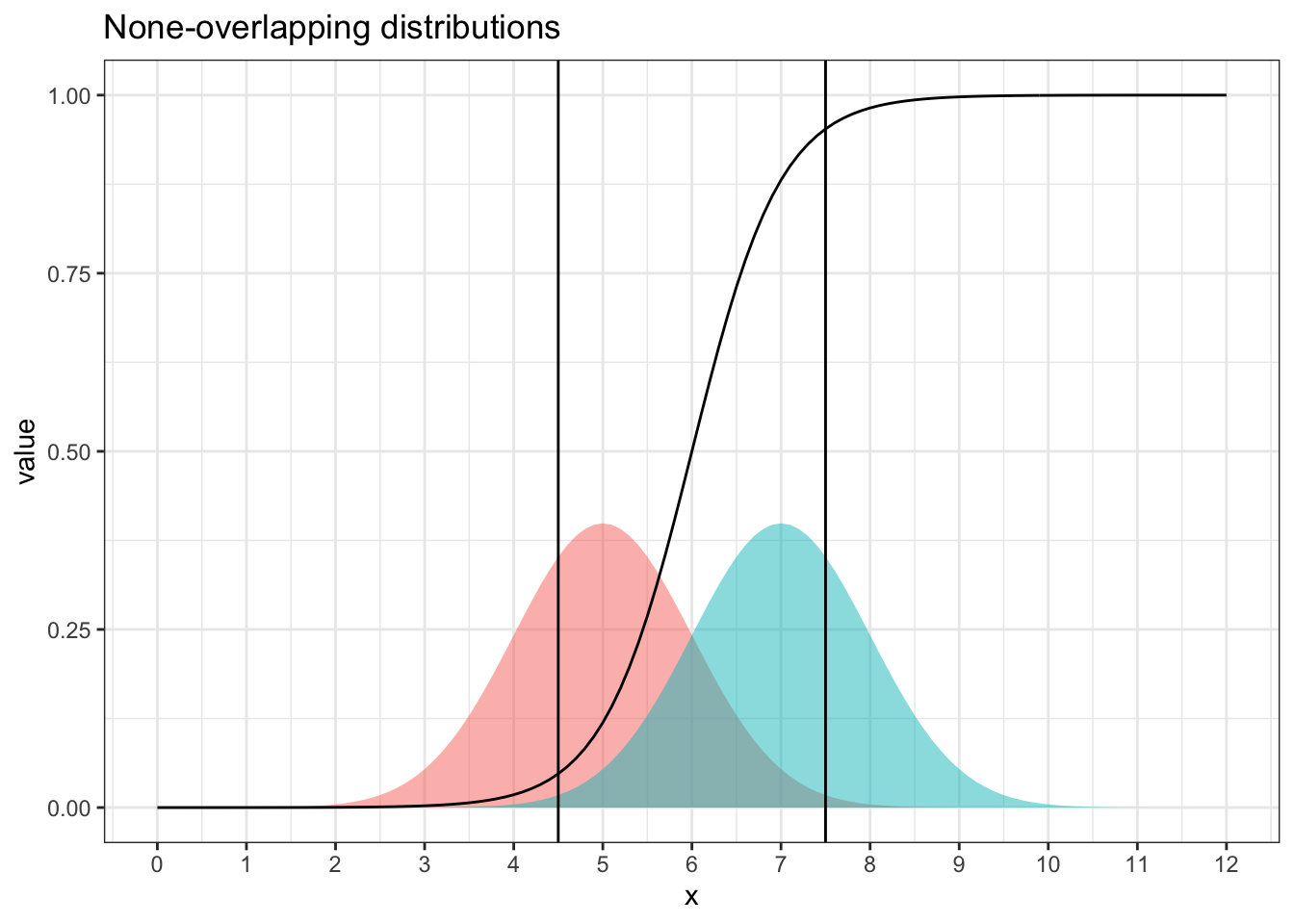
Figure 4.3: Two Distributions have large lack-of-overlapping areas with propensity function (of being from the distribution on the right). area outside the two vertical lines have propensity scores close to 0 or 1, indicating poor matching and high variance.
Figure 4.3 shows an example of two distribution that are apart. Outside of the central region between 4.5 and 7.5, propensity scores are less than 0.05 or larger than 0.95. A 0.05 propensity score means a 5:95 sample size ratio between the two distributions, and 0.95 propensity means 95:5. Either case shows a drastically imbalanced sample ratio.
The problem of highly imbalanced sample ratio? High variance! For two sample t-test, since the variance of the \(\Delta\) is proportional to \[ \frac{\sigma_T^2}{N_T}+\frac{\sigma_C^2}{N_C} \] where \(\sigma_T\) and \(\sigma_C\) are standard deviation of the treatment and control distribution. For illustration purpose, let’s assume the two standard deviations are the same. Then the variance of the \(\Delta\) is proportional to the sum of inverse \[ \frac{1}{N_T}+\frac{1}{N_C}. \] For a fixed total size \(N = N_T+N_C\), Figure 4.4 plots the sum of inverse as a function of the proportion of \(N_T\). We see that it is smallest when \(N_T = N_C\) and increase to infinity when \(N_T/N\) is either close to 0 or 1.
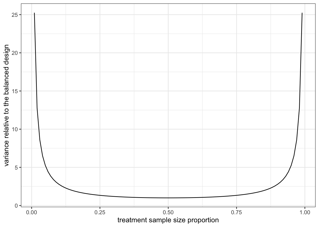
Figure 4.4: \(1/N_T+1/N_C\) as function of \(N_T/N\) when \(N=N_T+N_C\) is fixed.
The connection to matching is obvious. Since the purpose of exact matching or propensity matching is such that for each matching stratum, the observed data are as if they were from a conditional randomized experiments where treatment and control are randomized according to \(e(X):(1-e(X))\) ratio. We estimate the conditional average treatment effect (CATE) for each stratum and then aggregate to the ATE. The variance of ATE depends on variance of each CATEs. If one of it has high variance, the ATE will also be impacted. If some strata have \(e(X)\) close to 0 or 1, the variance of the corresponding CATE will be much larger than those stratum where \(e(X)\) is close to 1/2. Variance of ATE will be large and dominated by a few very large variances contributed by those small number of strata.
In the extreme case of \(e(X)\) equals 0 or 1, the matching fails completely. There exist either treatment group observations, or only control group observations, not both. This is equivalent to running a 100% vs. 0% randomized experiment and it is obvious in this total none-overlapping case that we cannot estimate the causal effect from only treatment or control observations.
Equivalently we can reach to the same conclusion that \(e(X)\) close to 0 or 1 leads to high variance of the IPW estimator (4.28) using the variance formula (4.23).
There is no silver bullet to overcome the lack-of-overlapping/none-overlapping problem. Practically solutions can be categorized into two orthogonal directions.
- Remove observations with propensity scores close to 0 or 1.
- Modify the propensity score model by removing some covariates from \(X\).
- Change the weights explicitly.
For the first approach, throwing away observations means we give up on estimating the average treatment effect for the whole population. For those regions where the propensity scores under the current model is close to 0 or 1, as we explained above, estimating CATE for these strata requires a lot of observations and is very inefficient because either treatment or control will only be a very small proportion of the sample. By leaving these strata out of the picture, we leave ourselves with an estimator that only estimates the average treatment effect on the well-overlapped region — a biased estimator if our goal is average treatment effect for whole population. But this biased estimator has much smaller variance. In other words, we are trading off variance with bias. Moreover, the bias here is explicitly known as not accounting effect from those lack-of-overlapping areas.
For the second approach, why can we modify the propensity score model by removing some covariates? The theory of propensity score and IPW does not mandate that there is only one propensity score model. In fact, there can be infinitely many. All we need is that the covariates \(X\) satisfies the conditional unconfoundedness condition \[ (Y(1),Y(0))\perp \! \! \! \! \perp Z | X . \] Imagine there exists a smallest set of covariates \(X^*\) satisfying the above condition. If we remove any one covariate from \(X^*\), the condition will fail. But it is possible that we can still add more covariates into the set \(X^*\) and still maintains the conditional independence condition.
The effect of adding more covariates? Potential more prediction power for \(Z\) given \(X\)! However, unlike traditional supervised learning problem where more prediction power is better, in propensity modeling, more prediction power leads to more propensity scores close to 0 or 1 — a nightmare for variance consideration. On the contrary, randomized experiments with a balanced treatment allocation (50% vs. 50%) corresponds to a propensity score being exactly 0.5 and there is no prediction power of any covariate set \(X\) to the treatment assignment \(Z\) since assignment is purely random. But randomized design using balanced assignment provides the best case scenario for estimating average treatment effect. Therefore, the purpose of propensity modeling is not for predicting treatment assignment \(Z\). Its real intention is for providing the correct weight for IPW estimation or simply dimension reduction for matching. Pursuing prediction accuracy when modeling propensity score does not help and to the contrary it only leads to high variance. This is a fundamental difference between propensity modeling and predictive modeling.
As an illustration, in the kidney stone example in Table 2.1 of Chapter 2, suppose the size of the stone is the only confounder needed to meet the conditional unconfoundedness requirement. Suppose treatment B is only offered in limited locations. In this case, knowing location information of a patient can greatly improves prediction power for which treatment a patient will choose. For patient outside of these limited locations, she can only pick treatment A, and we can 100% accuracy if our goal is to predict \(Z\). When conditioning on both kidney stone size and location, for these locations where treatment B is not available, there is of course no treatment B observations. In other words, keeping location as covariate to condition on leads to none-overlapping strata. But if kidney stone size alone meets the conditional unconfoundedness condition, we only need to condition on kidney stone size. Without location in the propensity score model, we no longer get extreme scores like 0 or 1.
The central issue here is how do we know whether a set of covariates \(X\) satisfies conditional unconfoundedness. Unfortunately there is no test. In practice, it is usually safer to put more covariates at first^[To the surprises of many, it is not true that it is safe to pick as many covariates as possible. Sometimes conditioning on certain covariates may create confoundness! We then check whether we get extreme propensity scores and as a result need to throw away some covariates that have high prediction power for assignment but at the same time deemed to be low in confounding effect. Of course the judgment of whether a covariate is likely to have confounding effect or not is subjective and with each covariate removed we are running under greater risk of missing confounding effect so the propensity scores are biased. In this sense, removing covariates should be justified as trading confidence in unbiasedness for reducing variance. But at least these subjective choices can be clearly documented so that the assumptions are part of the results.
For the third approach, Li, Morgan, and Zaslavsky (2018) proposed to use weight proportional to \(1-e(X)\) for treatment and \(e(X)\) for control. Comparing to the weights in IPW where treatment weight is proportional to \(1/e(X)\) and control weight proportional to \(1/(1-e(X))\), these new weights will never explode even for \(e(X)\) close to 0 and 1 (these will get very small weights). Intuitively, this has the similar effect as if we remove those non-overlapping region of \(X\). Li, Morgan, and Zaslavsky (2018) call this overlap weight and showed that this weighting method unbiasedly estimate the average treatment effect under a reweighted population distribution of \(X\) by putting an weight of \(e(X)(1-e(X)\). That is, by using the overlap weight, we explicitly avoid the task of estimate the ATE under the true population distribution where non-overlapping issue exists; instead, we give small weights to non-overlapping areas and larger weights to overlapping areas to mitigate the issue of exploding weight. This can be seen as a soft version of the first approach where we give 0 weight for observations in non-overlapping areas.
4.11 Other Propensity Score Modeling Methods
Propensity scores \(P(Z=1|X)\) have to be learned from the data unless the data generation process is known as in randomzed experiments. Traditional approach takes the data pairs \((Z,X)\) and fit a probabilistic model such as a logistic regression model to predict the propensity scores. These parametric models are subject to model mis-specification. This is why in practice directly using IPW with logistic regression fitted propensity score often give unreliable results and people will either use matching on propensity score and use propensity score merely as dimension reduction tool instead of weights, or use doubly robust estimation.
Imai and Ratkovic (2014) realized that the MLE of a logistic regression model for propensity modeling is equivalent to minimize the imbalance of the sigmoid function’s partial derivative with respect to the parameter (sigmoid function is a function of covariate \(X\) and model parameter) between treatment and control. Since covariate \(X\) is not affected by treatment, ideally any function of covariate \(X\) should be balanced. Why just optimize for this partial derivative of a sigmoid function?
In light of this, Imai and Ratkovic (2014) proposed to fit any parametric propensity score model using method of moments for a set of balancing equations. This covariance balancing propensity score (CBPS) method generalized logistic regression and other parametric models by making the optimization goal of the model fitting explicit in forms of balancing arbitrary functions of \(X\).
This idea of direct optimization of covariate balance make the problem of propensity score modeling into a constrained covariate blancing optimization problem, which can also be extended to nonparametric model. For instance, Hainmueller (2012) proposed entropy balancing to choose individual weights directly without a parametric model. Also see Athey, Imbens, and Wager (2018).
The idea of potential outcome is first introduced by J. Neyman in his 1925 master thesis on application of randomized experiments in agriculture where he talked about “potential yield.”↩︎
The name “ignorability” stems from the missing data view. It means the missing data mechanism can be ignored and we can treat them to be missing completely at random. See Section 4.5.↩︎
For this reason some authors prefer the name complete unconfoundedness to emphasize no confounders are left outside.↩︎
This proof is borrowed from Pearl (2009) with notation changes↩︎
Actually independence is not required but variances of Monte Carlo estimators will be harder to estimate without independence.↩︎
Here and after \(\mathrm{E}\) is taken under the complete data probability measure \(P^*\) unless otherwise explicitly specified.↩︎