Chapter 3 Randomized Experiment
What could an experimental physicist do if she wants to compare two experiment conditions? Simple. She just need to run two experiments under both conditions and then compare the outcomes. In Table 2.1 there are two different treatments of kidney stones, A and B. Pick any patient in Table 2.1. If a patient took treatment A, we observe the outcome of treating the patient with A. It is impossible for us to rewind the time and force the patient to take treatment B and observe the outcome. Even if we could, what we really want to observe is the outcome of treating this patient with treatment B if he or she chose treatment B under no coercion. The same situation applies to patients took treatment A and we are not be able to know what treatment B would do to them. These hypothetical outcomes, not observed and also impossible to observe, are called the counterfactuals.
Counterfactuals are like ghost observations and cannot be directly used in any calculation. They plays a pivotal role in the potential outcome framework. Theories of the potential outcome framework center around the question of whether and how can we infer statistical quantities, e.g. mean, of a counterfactual by only using observed outcomes. Potential outcomes and its related theories are our topics for the next chapter. But long before the advent of potential outcome framework and even the existence of statistics as a discipline, the idea of randomized experiment was already being used.
Take the kidney stone treatment example. If we do not allow patients to self-select their treatment. Instead, we design a split of patients into two groups receiving treatment A and B. If the split is done such that the only difference between the two groups is the treatment they use and all other things being equal, then any difference between outcomes of the two groups can only possibly be caused by the difference in the treatments they received. In other words, the comparison of the two groups should be a fair comparison immune to any systematic selection bias.
Randomization is the simplest strategy to ensure an all-other-thing-being-equal splitting. It is a form of intervention that echos the definition of causal effect as the result of change through intervention. Inferring causal effect by means of randomization is also called randomized experiment, or controlled experiment. We learn the effect of change through intervention by really doing intervention, similar to scientists running experiments by changing experiment conditions in a lab. The subtle difference is randomization does not allow us to observe the counterfactuals under different conditions directly. Instead, it relies on the magic spell “all other things being equal.” Arguments using the power of “all other things being equal” are extremely simple to almost being obvious. Fisher, whose work in early 1920s popularized the idea of randomized experiment, believed randomization and more generally the idea of permutation to be obvious to anyone and treated them as examples of his “logic of inductive science.” As form of logic, he believed no formal statistics or mathematics is needed to convey the idea to any rational person. Indeed, in logic, Ceteris paribus is the Latin phrase for “all other things being equal” and any conclusion based on using this argument is called a cp law.
Different randomization mechanisms can achieve all-other-thing-being-equal. In all randomization mechanism we consider the case of only two groups. Extension to more than two groups is straightforward. For two group cases, we often call one group treatment and the other control. Define assignment indicator \(Z\) as \(Z=0\) for being assigned to the fist group (control) and \(Z=1\) for being assigned to the second group (treatment). Although different randomization mechanisms all achieve the requirement of all-other-thing-being-equal. The choice of randomization mechanism has an implication in the data generating process underneath the collected observations and has an impact on the following statistical analysis.
3.1 Complete Randomization
Suppose there are \(N\) subjects in total and we want to split them into two groups of sizes \(M\) and \(N-M\). All we need to do is to sample \(M\) subjects out of \(N\) without replacement. Each patient have the same probability \(M/N\) of being assigned to the first group and probability \(1-M/N\) to be assigned to the second group.
Complete randomization is closely connected to the idea of permutation. One way of implementing complete randomization would be permute the \(N\) subjects into a random order and assign the first \(M\) subjects to the first group and the rest to the second.
Complete randomization ensures the size of each group to be fixed. However, assignment \(Z\) for different subjects are not independent. To see that, \(Z = 1\) for one subject reduces the chance of \(Z=1\) for another subject because of the fixed size of treatment and control. For \(i^{\text{th}}\) and \(j^{\text{th}}\) subject, \[\begin{align*} \mathrm{Cov}(Z_i, Z_j) & = \mathrm{E}(Z_i Z_j) - \mathrm{E}(Z_i)\mathrm{E}(Z_i) \\ & = \frac{M}{N}\frac{M-1}{N-1} - \left( \frac{M}{N} \right)^2 < 0. \end{align*}\]
3.2 Independent Randomization
Complete randomization requires experimenters to know the total size and desired sizes for each groups at the randomization stage. In many applications, subjects were recruited on an ongoing basis. For these cases, randomization can also be done by drawing a group label from a multi-class Bernoulli distribution independently for each subject.
Suppose we need to split \(N\) subjects into K groups with probabilities \(p_1, \dots, p_K\), \(\sum_k p_k = 1\). For each subject, we draw the group label \(L\) from the distribution following \[ L = k, \quad \text{with probability } p_k, \quad k = 1,\dots, K. \]
Unlike in complete randomization, assignment indicator \(Z\) for different subjects are by design independent. Also, the group sizes \(N_1,\dots,N_K\) are no longer fixed numbers but a random vector from multinomial distribution \[ (N_1,\dots,N_K) \sim \text{Multinom}(N, p_1,\dots,p_K). \]
Independent randomization is also called Bernoulli trial as each assignment is an independent Bernoulli random variable.
3.3 Clustered Randomization
Often, treatments are assigned at the level of each subject. This is not always the case nor is it always desired. For example, when doing an experiment to study effect of certain education method, randomizing each individual student is not possible and randomizing each classroom is more appropriate. Randomizing clusters of subjects still satisfies all-other-things-being-equal. Either complete randomization or independent randomization can be used to randomize clusters.
Clustered randomization is commonly used when social spillover or interference effect exists. In the education method example above, since students are interacting with each other and even might form study groups, it is possible that the effect of a new education method on a student will also be affected by assignments of other students he or she closely interacts with. In case like this, if we can cluster students such that inter-cluster level interference is negligible, then a clustered randomization should be used.4
Clustered randomization highlights the distinction of two different units: randomization unit and analysis unit. Analysis unit is the unit at which we want to infer causal effect. Randomization unit is the unit at which randomization is performed. Randomization unit has to be defined equal or less granular than the analysis unit. This means randomization can be applied on clusters of analysis units but within each analysis unit randomization of sub-analysis unit level does not make sense. To see this, if a sub-analysis unit is used for randomization, then each analysis unit could experience both treatment and control and can no longer belong to only one treatment group.
3.4 Analysis of Randomized Experiments as Two Sample Problem
Although randomization experiment provides a straightforward method to infer causal effect and the all-other-thing-being-equal argument is obvious to most minds, the analysis of randomized experiments remains a statistical problem. Rigorous analysis of randomized experiment requires using a causal model such as potential outcomes framework. Potential outcome framework will be our main topic in the Chapter 4, where we will show randomization satisfies a condition called “ignorability” or “unconfoundedness” under which naive comparison of different treatment groups leads to an unbiased estimation of causal effect — mathematically justifying the all-other-thing-being-equal logic. Here we briefly go through a widely used practice simply treating the analysis of randomized experiments as a special application of the two sample problem.
The two sample problem concerns with two independent samples drawn from two distributions, and a typical interest is to compare the means of the two. Let \(X, X_1,\dots,X_N\) and \(Y, Y_1,\dots,Y_M\) are i.i.d. random variables. That is, we observed \(N\) i.i.d. observations having the same distribution as \(X\) and \(M\) i.i.d. observations as \(Y\). We are interested in the difference of the two means \[\begin{equation*} \delta = \mathrm{E}(Y) - \mathrm{E}(X). \end{equation*}\]
\(\delta\) can be unbiased estimated by the estimator \[\begin{equation*} \Delta = \overline{Y} - \overline{X}. \end{equation*}\]
When \(N\) and \(M\) are small, the distribution of \(\Delta\) is hard to track down. If we further assume \(X\) and \(Y\) are both normally distributed, then we know \(\Delta\) is also normally distributed and we should focus on estimating its variance. Since \(X_i\) and \(Y_i\) are independent, \[\begin{align*} \mathrm{Var}_\text{TS}(\Delta) & = \mathrm{Var}(\overline{Y})+ \mathrm{Var}(\overline{X}) \\ & = \frac{\mathrm{Var}(Y)}{M} + \frac{\mathrm{Var}(X)}{N}, \end{align*}\] where the subscript \(TS\) stands for two sample and \(\mathrm{Var}(Y)\) can be unbiasedly estimated using sample variance formula \[ \widehat{\sigma}_Y^2 = \frac{\sum_i (Y_i - \overline{Y})^2}{M-1} \] given i.i.d. \(Y_i\) and similarly \(\widehat{\sigma}_X^2\) for \(\mathrm{Var}(X)\). \(M-1\) here is merely for finite sample unbiasedness and is often replaced by \(M\) unless \(M\) is very small.
Let’s denote the estimated \(\mathrm{Var}_\text{TS}(\Delta)\) by \(\widehat{\sigma}_\text{TS}^2\), \(\frac{\Delta - \delta}{\widehat{\sigma}_\text{TS}}\) follows a standard normal distribution if we ignore the fact that \(\widehat{\sigma}_\text{TS}\) is an estimator and not same as the true standard deviation of \(\Delta\). Indeed, when \(M\) and \(N\) are large, by the law of large number and the Slutsky’s theorem, \(\frac{\Delta - \delta}{\widehat{\sigma}_\text{TS}}\) converges in distribution to the standard normal distribution. When \(M\) and \(N\) are small, Gosset, under the name Student, showed that \(\frac{\Delta - \delta}{\widehat{\sigma}_\text{TS}}\) follows a t-distribution which has a heavier tail than standard normal distribution.5
With moderate to large number of samples, even without \(X\) and \(Y\) being normally distributed, \(\Delta\) and its standardized version \(\frac{\Delta - \delta}{\widehat{\sigma}_\text{TS}}\) will be approximately normal thanks to the central limit theorem (and Slutsky’s theorem for the normalized \(\Delta\)). Also in this case the t-distribution, with a degree of freedom over 30, is practically equivalent to a normal distribution.
The moderate to large sample case is also referred to as z-statistic, and z-test for the corresponding hypothesis test, as compared to t-test based on t-statistic. In practice this distinction is often (rightfully) ignored. The normal assumption on both \(X\) and \(Y\) for the small sample case is too strong to meet in most applications. Efforts often have to be made to transform observations into a normal-like distribution. This is not necessary for large sample case as long as the central limit theorem kicks in. This is why z-statistic and z-test are much more useful in practice. However because t-statistic automatically turns into a z-statistic when degree of freedom is large. People often keep using the name t-statistic and t-test.
For moderate to large sample case, a \(1-\alpha\) two sided confidence interval is \[ \Delta \pm z_{\alpha/2} \widehat{\sigma}_\text{TS}\,, \] where \(z_{\alpha/2}\) is the \(1-\alpha/2\) quantile of the standard normal distribution.
Correspondingly, a two-sided z-test for the null hypothesis \(H_0: \delta = 0\) is to reject \(H_0\) when \[ \frac{|\Delta|}{\widehat{\sigma}_\text{TS}} \ge z_{\alpha/2}\,. \]
For a randomized experiment with binary treatment, by the all-other-thing-being-equal argument, the causal effect of the treatment becomes the difference between the two groups. Comparing the treatment group and the control group seems to naturally fit into a two sample problem. \(\Delta\) becomes an unbiased estimator for the causal effect for the mean — the average treatment effect. However, there are a few notable differences.
Unlike the standard two sample problem, where the data-generating-process is such that we sample i.i.d. observations from treatment and control groups separately and independently. Data-generating process in a randomized experiments is more complicated and relies on two things: the randomization mechanism and also the causal estimand.
For complete randomization, the data-generating process involves two steps, first step is to sample \(N+M\) units for the experiment with their counterfactual pair \((Y(1),Y(0))\), and the second step is the permutation such that \(N\) units are assigned to control and \(M\) to the treatment. The observation is \(Y(1)\) if assigned to treatment and \(Y(0)\) if control. The first step is optional as some researchers such as Neyman prefer to assume \(N+M\) units are given and only focus on the average treatment effect on this set of \(N+M\) units (This is called sample average treatment effect SATE, comparing to population average treatment effect PATE). In this case observations are not independent within each group or across groups due to sampling without replacement. The randomness in a complete randomized experiments are only due to the assignment randomization. Considering population average treatment effect adds the first step of sampling \(M+N\) units into the picture but it draws from a single distribution of counterfactual pairs rather than from two distributions independently as in the independent two sample problem.
For independent randomization and for population average treatment effect, the data-generating-process is first independently toss a coin as the treatment assignment process and then independently draw from treatment distribution or control distribution based on the treatment assignment. This does provide i.i.d. observations for both treatment group and control groups, and also guarantees independence between the two groups. In the classic Bernoulli trial introduced above, we fix the total sample size \(M+N\) and \(M\) (and \(N\)) is not a fixed number but rather from a Binomial distribution. If instead of population average treatment effect, the sample average treatment effect is desired, the data-generating-process is again different. \(M+N\) counterfactual pairs are assumed to be given. For each of them, we independently assign treatment or control to decide \(Y(1)\) or \(Y(0)\) to observe.
Despite the differences, two sample t-test or z-test are often used in practice for both complete randomization design and independent randomization design. Is this a huge mistake that practitioners have been making? Fortunately, the conclusion is this practice is totally fine and we will now explain.
We first look at the complete randomization design. Recall it differs from independent sampling because treatment assignments of units are negatively correlated with each other. Typically, if we have sum of negatively correlated random variables, we expect the variance of the sum to be smaller than the independent case because \[\begin{align*} \mathrm{Var}(\sum_i Y_i) & = \sum_i \mathrm{Var}(Y_i) + \sum_i \sum_{j \neq i}\mathrm{Cov}(Y_i, Y_j) \\ & < \sum \mathrm{Var}(Y_i) \end{align*}\] if \(\mathrm{Cov}(Y_i, Y_j) < 0\). This suggests that the variance estimation \({\widehat{\sigma}_X^2}/N\) and \({\widehat{\sigma}_Y^2/M}\) are over-estimating the true variance of \(\mathrm{Var}(\overline{X})\) and \(\mathrm{Var}(\overline{X})\). However, because of the same negative correlation, \[ \mathrm{Var}(\Delta) = \mathrm{Var}(\overline{Y}-\overline{X}) > \mathrm{Var}(\overline{Y})+\mathrm{Var}(\overline{X}), \] leading to under-estimation of \(\mathrm{Var}(\Delta)\) when ignoring the dependency between \(\overline{Y}\) and \(\overline{X}\).
Put these two ``errors’’ together, when we pretend two samples are i.i.d. from its own distribution and apply two sample t-test or z-test with \[ \mathrm{Var}_\text{TS}(\Delta) = \mathrm{Var}(\overline{Y})+ \mathrm{Var}(\overline{X}), \] we are over-estimating the variance of both component on the RHS, but also missing a positive covariance between \(\overline{Y}\) and \(\overline{X}\), leading to under-estimation of the LHS. It is unclear \(\mathrm{Var}_\text{TS}(\Delta)\) is over-estimating or under-estimating the true variance because the two opposing corrections without exact derivation.
Imbens and Rubin (2015) analyzed the exact variance formula for completed randomized experiments, for both sample average treatment effect (SATE) and population average treatment effect (PATE). The results are comforting. For PATE, they showed that \(\mathrm{Var}_\text{TS}(\Delta) = \frac{\mathrm{Var}(Y)}{M} + \frac{\mathrm{Var}(X)}{N}\) turns out to be the correct variance of \(\Delta\). In other words, the two errors in different directions strike a perfect balance and the sum of the two has no error — the two sample problem, under a totally different data-generating-process, produces the correct variance. For SATE, the true variance is always smaller than the two sample variance \(\mathrm{Var}_\text{TS}(\Delta)\). Imbens and Rubin (2015) showed the correction term relies on the variance of individual treatment effect for the \(M+N\) units. When there is no individual treatment effect variation, the correction term is \(0\) so \(\mathrm{Var}_\text{TS}(\Delta)\) again is exact. In general there is no estimator for the correction term available because individual treatment effects are not observable. \(\mathrm{Var}_\text{TS}(\Delta)\) remains an close upper bound.
Now we look at the independent randomization. Independent randomization for PATE is closer to the data-generating-process of two sample t-test and z-test, except that sample sizes \(M\) and \(N\) are not fixed but random. In the analysis of two sample problem when sample sizes are fixed, for \(\mathrm{Var}_\text{TS}(\Delta)\) we used the fact \[ \mathrm{Var}(\overline{Y}) = \frac{\mathrm{Var}(Y)}{M}. \] When \(M\) is random, the above is not correct. We offer two justifications that we can pretend sample sizes are fixed in practice.
The first justification is using large sample theory and the second justification is conditional test.
Applying the conditional variance formula leads to \[\begin{align*} \mathrm{Var}(\overline{Y}) & =\mathrm{E}\left( \mathrm{Var}(\overline{Y} | M) \right) + \mathrm{Var} \left( \mathrm{E} (\overline{Y} | M) \right ) \\ & = \mathrm{E}\left( \mathrm{Var}(Y)/M \right). \end{align*}\] The last equality is because \(\mathrm{E} (\overline{Y} | M) = \mathrm{E}(Y)\) is a constant with zero variance. Moving the constant \(\mathrm{Var}(Y)\) out of the last expectation, \[\begin{equation} \mathrm{Var}(\overline{Y}) = \mathrm{Var}(Y)\times \mathrm{E}(\frac{1}{M}). \tag{3.1} \end{equation}\] We see that the correct variance of \(\overline{Y}\) depends on \(\mathrm{E}(\frac{1}{M})\) (and \(\mathrm{E}(\frac{1}{N})\) for \(\overline{X}\)). (Technically the expectation here is a conditional expectation given \(M>0\) and \(N>0\) because the comparison does not make sense if only one group gets observations.) For independent randomization, \(M\) and \(N\) follows binomial distribution. By central limit theorem \(M\) is \(O(\sqrt{M})\) away from its expectation \(\mathrm{E}(M)\), and for \(N\) similarly. As \(M+N\) increases and when \(M\) and \(N\) are both moderately large, \(\frac{1}{M}\), \(\mathrm{E}(\frac{1}{M})\) and \(\frac{1}{\mathrm{E}(M)}\) are all close enough to be practically equivalent and the same goes for \(N\). This is why for independent randomized experiment, in almost all applications we can treat the sample sizes as if they are fixed numbers. A proof of this requires using central limit theorem with the delta method and can be found in Section 11.2. The result holds not only for binomial distribution, but more general for any \((M,N)\) abiding the central limit theorem. Here we use simulation to illustrate the point. Figure shows the distribution of the ratio of \(1/M\) to \(\frac{1}{\mathrm{E}(M)}\) when \(M\) is from a binomial(K,0.5) distribution with increasing \(K = M+N\). The vertical line is the ratio of \(\mathrm{E}(\frac{1}{M})\) to \(\frac{1}{\mathrm{E}(M)}\). We see with \(K = 1,000\), the ratio of \(\mathrm{E}(\frac{1}{M})\) to \(\frac{1}{\mathrm{E}(M)}\) is already very close to 1. Moreover, \(1/M\) is almost always within 10% relative error for \(\frac{1}{\mathrm{E}(M)}\). A 10% relative error for variance only translate to 5% error for the standard error, and for the test statistics. This error is even smaller with larger sample sizes.
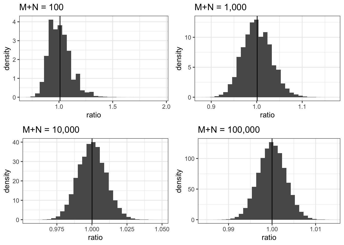
Figure 3.1: Ratios of \(1/M\) and \(\frac{1}{\mathrm{E}(M)}\) as \(N+M\) increases from \(100\) to \(100,000\). vertical line is the ratio of \(\mathrm{E}(\frac{1}{M})\) to \(\frac{1}{\mathrm{E}(M)}\).
The conditional test perspective offers another justification regardless of sample size. Note that the sample size \(M\) and \(N\) are irrelevant to our interest of comparing two distributions. \(M\) and \(N\) are called nuisance parameters. We can partition the data-generating-process into two components, one that involves the parameter of interest, and one that only involves nuisance parameters. One can argue that only the first part contains information for the inference of the parameter of interest. And the second part only adds noises that contains no useful information.
By this argument, for the purpose of two sample comparison, we can condition on \(M\) and \(N\) by taking them out of the data-generating-process, meaning that we change the natural data-generating-process into a conditional version where we fix not only \(N+M\) but also \(N\) and \(M\). After fixing \(N\) and \(M\), the conditional data-generating-process reduces to the the two sample comparison and we can treat both \(X_i\) and \(Y_i\) are i.i.d.6
The last case to justify is independent randomization for SATE. After conditioning on sample sizes, the conditional data-generating-process is the same as complete randomization for SATE. And we have already justified using two sample t-test or z-test for this case.
The analysis of randomized experiments are much sophisticated and richer than two sample problem described in this section. Other randomization mechanism such as cluster randomization and stratified randomization poses different data-generating-processes where \(\mathrm{Var}_\text{TS}(\Delta)\) could deviate from the true variance of \(\Delta\) a lot. Also, our causal estimand of interest might not be as simple as the difference in the mean. Moreover, there exists better experiment design and more accurate estimator (smaller variance) for average treatment effect. Randomized experiments have huge application in the Internet era for online industry, where it got a new name called A/B testing (or A/B/n testing for more than one treatment). We will see randomized experiments again in later chapters on randomized experiments with a focus on online application.
Technically it is a Welch’s t. Student’s original t-statistic assumes common variance of \(X\) and \(Y\) and used a pooled variance estimator.↩︎
In Bayesian statistics, we always condition on observations and infer the conditional distribution of the parameter of interest given observations. There is no such issue as nuisance parameter. In Frequentist statistics, conditional test often improves statistical power because it removes noises from nuisance parameters.↩︎